Basic signal detection theory model

import os

if "KERAS_BACKEND" not in os.environ:
    # set this to "torch", "tensorflow", or "jax"
    os.environ["KERAS_BACKEND"] = "jax"

import matplotlib.pyplot as plt
import numpy as np

import keras
import bayesflow as bf

from scipy.stats import norm

In this example we will fit a basic signal detection theory model:

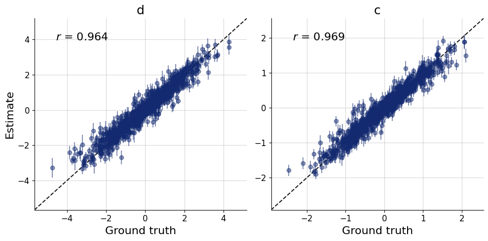
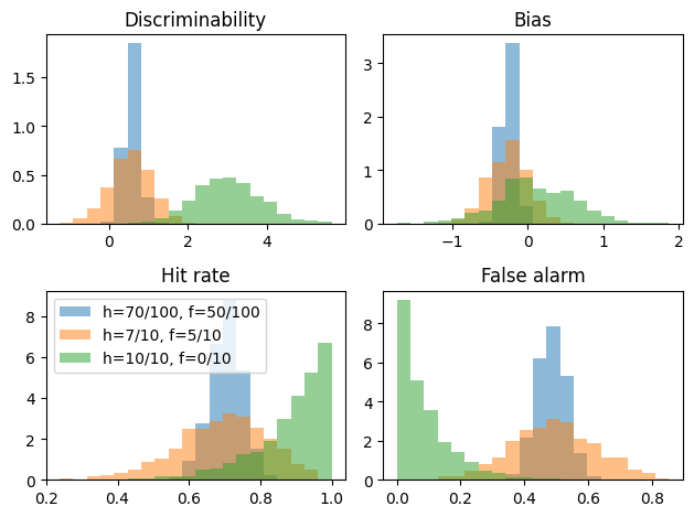
\[\begin{equation} \begin{aligned} d & \sim \text{Normal}\left(0, \sqrt{2}\right) \\ c & \sim \text{Normal}\left(0, \sqrt{\frac{1}{2}}\right) \\ \theta_h & \leftarrow \Phi\left(\frac{d}{2} - c\right) \\ \theta_f &\leftarrow \Phi\left(- \frac{d}{2} - c\right) \\ h & \sim \text{Binomial}(\theta_h, n_\text{signal}) \\ f & \sim \text{Binomial}(\theta_f, n_\text{noise}), \\ \end{aligned} \end{equation}\] where \(h\), \(f\) are the number of hit rates and false alarms, out of \(n_\text{signal}\) and \(n_\text{noise}\) trials, respectively. We will estimate the distriminability \(d\) and bias \(c\). During the inference stage we will be also interested in the implied hit rate \(\theta_h\) and false alarm rate \(\theta_f\).

Simulator

Setting up the simulator is straightforward. We wish to be able to make inferences for different numbers of trials, and so we will vary that as a context variable.

def context():
    return dict(n = np.random.randint(low=5, high=120, size=2))

def prior():
    return dict(
        d = np.random.normal(0, np.sqrt(2)),
        c = np.random.normal(0, np.sqrt(1/2))
    )

def likelihood(d, c, n):
    # compute hit rate and false alarm rate:
    theta = norm.cdf([0.5 * d - c, - 0.5 * d - c])
    # simulate hits and false alarms
    x = np.random.binomial(n=n, p=theta, size=2)

    return dict(x=x)

simulator = bf.make_simulator([context, prior, likelihood])

Approximator

We will use a BasicWorkflow object to wrap up all necessary networks.

workflow = bf.BasicWorkflow(
    simulator=simulator,
    inference_network=bf.networks.CouplingFlow(),
    inference_variables=["d", "c"],
    inference_conditions=["x", "n"]
)

Training

history = workflow.fit_online(epochs=50, num_batches_per_epoch=200, batch_size=256)

Validation

test_data = simulator.sample(1000)

{'losses': <Figure size 1600x400 with 1 Axes>,
 'recovery': <Figure size 1000x500 with 2 Axes>,
 'calibration_ecdf': <Figure size 1000x500 with 2 Axes>,
 'z_score_contraction': <Figure size 1000x500 with 2 Axes>}

figs = workflow.plot_default_diagnostics(test_data=test_data, num_samples=500)

Inference

We are given three data sets (Lee & Wagenmakers, 2013):

1. \(h=70\), \(f=50\), \(n_{\text{signal}} = n_{\text{noise}} = 100\)
2. \(h=7\), \(f=5\), \(n_{\text{signal}} = n_{\text{noise}} = 10\)
3. \(h=10\), \(f=0\), \(n_{\text{signal}} = n_{\text{noise}} = 10\).

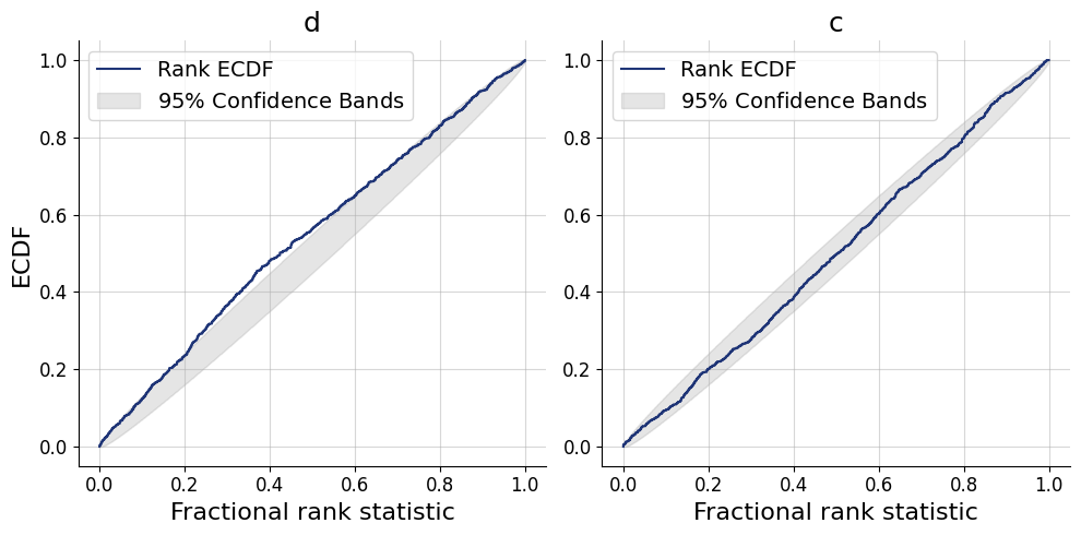
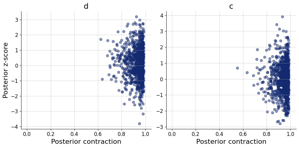
We can leverage the fact that we can make inferences for all three datasets at the same time, we will get an array of the posterior samples of \(d\) and \(c\) for each of the datasets.

inference_data = dict(
    x = np.array([
        [70, 50],
        [7, 5],
        [10, 0]
    ]),
    n = np.array([
        [100, 100],
        [10, 10],
        [10, 10]
    ])
)

posterior_samples = workflow.sample(conditions=inference_data, num_samples=1000)

def generated_quantities(c, d):
    return {
        "Discriminability": d,
        "Bias": c,
        "Hit rate": norm.cdf(0.5 * d - c),
        "False alarm": norm.cdf(-0.5 * d - c)
    }

posterior_samples = generated_quantities(**posterior_samples)

fig, axs = plt.subplots(2, 2)
axs=axs.flatten()

for index, (key, value) in enumerate(posterior_samples.items()):
    bins = np.histogram_bin_edges(value.ravel(), bins=20)
    for data_set in range(inference_data['x'].shape[0]):
        axs[index].hist(value[data_set].flatten(), alpha=0.5, density=True, bins=bins)
        axs[index].set_title(key)
axs[2].legend(['h=70/100, f=50/100', 'h=7/10, f=5/10', 'h=10/10, f=0/10'])
fig.tight_layout()

References

Lee, M. D., & Wagenmakers, E.-J. (2013). Bayesian Cognitive Modeling: A Practical Course. Cambridge University Press.