The seven scientists

Author

Šimon Kucharský

Published

May 6, 2025

Code

import os

if "KERAS_BACKEND" not in os.environ:
    # set this to "torch", "tensorflow", or "jax"
    os.environ["KERAS_BACKEND"] = "jax"

import matplotlib.pyplot as plt
import numpy as np
import bayesflow as bf

INFO:bayesflow:Using backend 'jax'

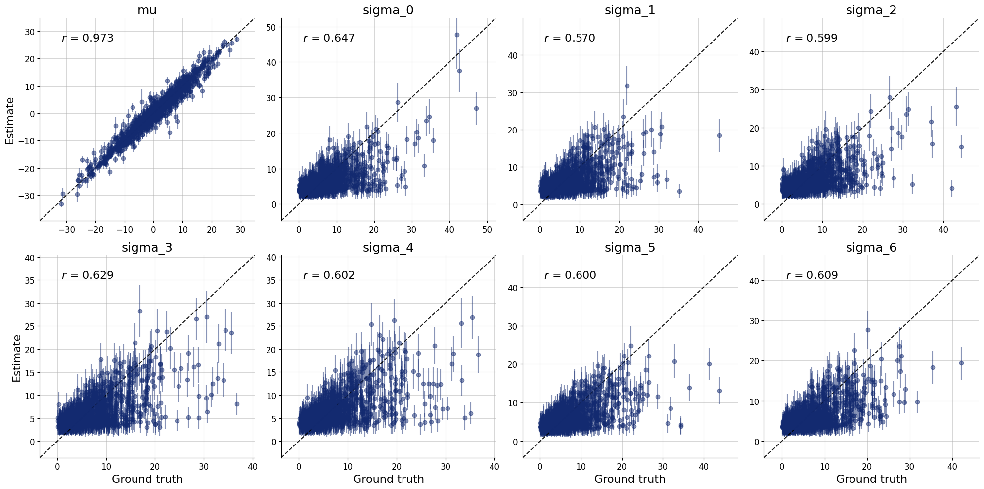
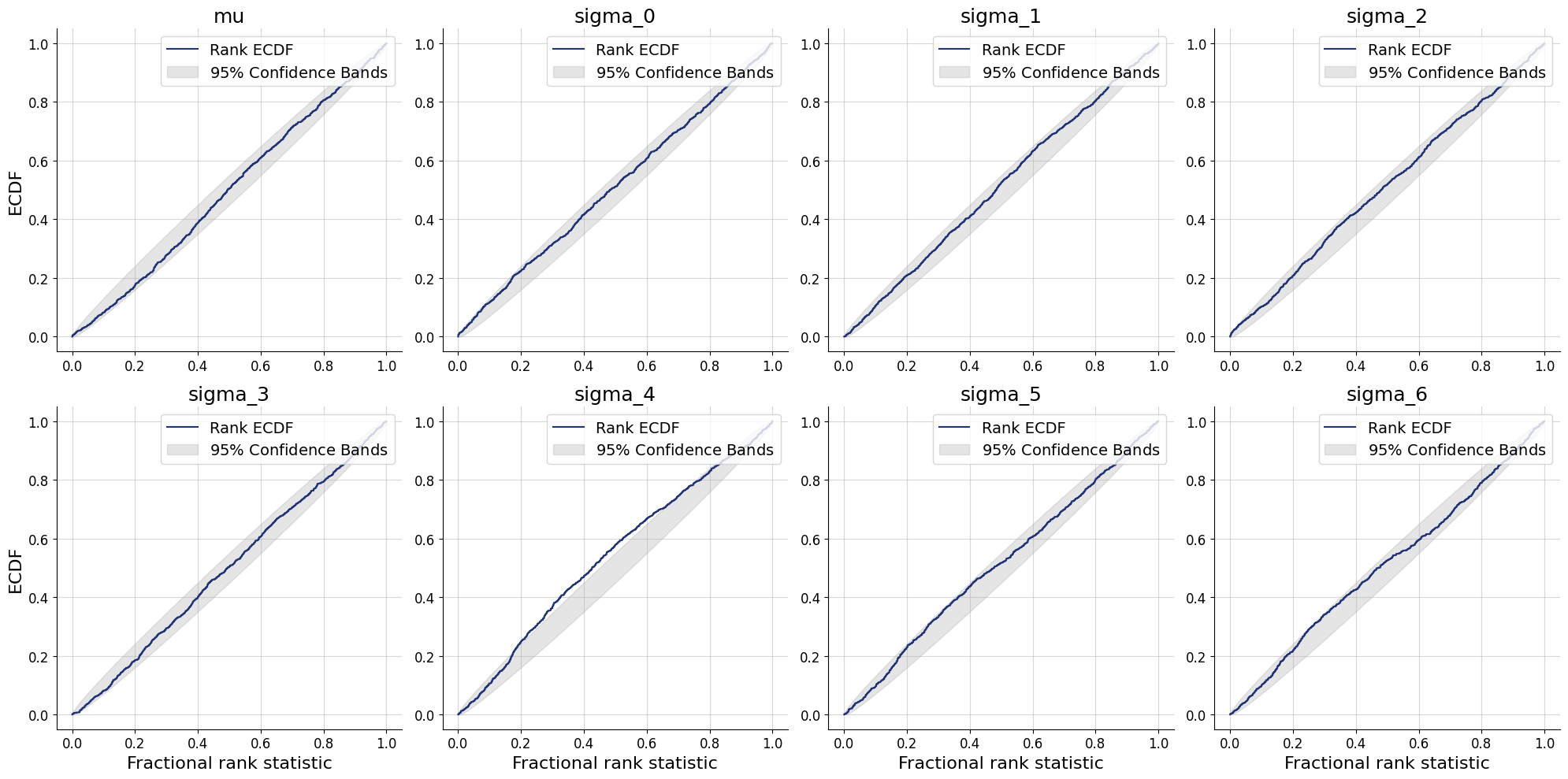
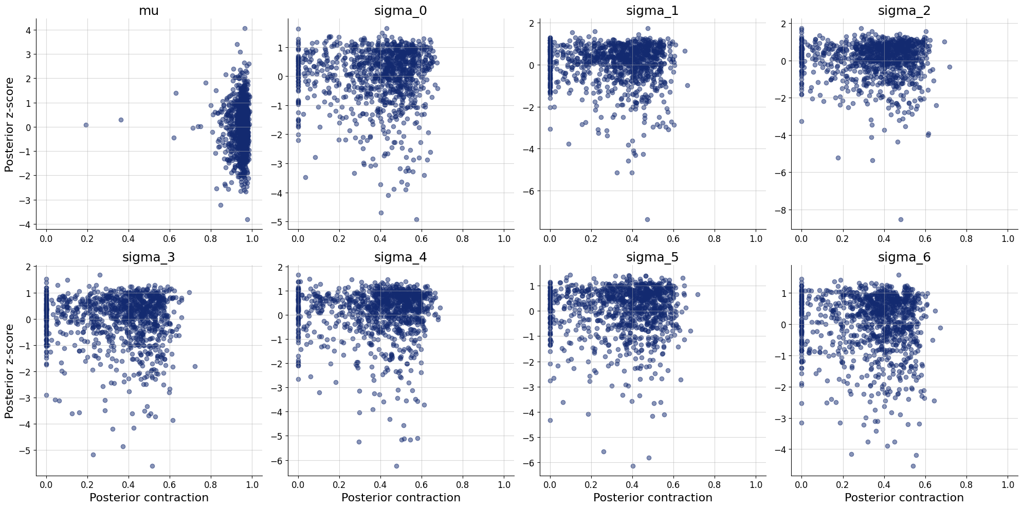
In this section we will estimate the experimental skills of seven scientists that measure the same quantity. We can reformulatted the original model as such:

\[\begin{equation} \begin{aligned} \mu & \sim \text{Gaussian}(0, 10) \\ \sigma_i & \sim \text{Gamma}(1.5, 5) \\ x_i & \sim \text{Gaussian}(\mu, \sigma_i), \end{aligned} \end{equation}\] where \(i \in (1, 2, ..., 7)\) is the index of the scientist.

Note that we put a prior on the measurement standard deviation rather than on the measurement precision. Further, instead of using the rather wide prior \(\text{Gamma}(0.001, 1000)\), we use a more restricted version. This prior still puts more mass on values close to zero, but does not generate extreme values that might cause numerical stability issues during data simulations. Similarly, we also reduced the variance of the prior on \(\mu\), as in the original example it appears unnecessarily large.

Simulator

Code

def prior():
    mu=np.random.normal(scale=10)
    sigma=np.random.gamma(shape=1.5, scale=5, size=7)

    return dict(mu=mu, sigma=sigma)

def likelihood(mu, sigma):
    x=np.random.normal(loc=mu, scale=sigma)
    
    return dict(x=x)

simulator=bf.make_simulator([prior, likelihood])

Approximator

Code

adapter = (
    bf.Adapter()
    .constrain(["sigma"], lower=0)
    .standardize(include=["mu", "sigma"])
    .concatenate(["mu", "sigma"], into="inference_variables")
    .rename("x", "inference_conditions")
    )

Code

workflow=bf.BasicWorkflow(
    simulator=simulator,
    adapter=adapter,
    inference_network=bf.networks.CouplingFlow()
)

Training

Code

history=workflow.fit_online(epochs=50, num_batches_per_epoch=200, batch_size=512)

Validation

Code

test_data=simulator.sample(1000)
figs=workflow.plot_default_diagnostics(test_data=test_data, num_samples=500)

Inference

Here we will compute the parameter estimates for the problem of seven scientists. Use them to answer the questions in the book (Lee & Wagenmakers, 2013).

Code

x=np.array([[-27.020, 3.570, 8.191, 9.898, 9.603, 9.945, 10.056]])
inference_data = dict(x=x)

Code

samples=workflow.sample(num_samples=2000, conditions=inference_data, split=True)

Code

workflow.samples_to_data_frame(samples).describe().transpose()

	count	mean	std	min	25%	50%	75%	max
mu	2000.0	8.364841	1.850573	1.976640	7.165722	8.493637	9.682344	14.703032
sigma_0	2000.0	20.852479	6.511639	8.009318	16.441570	19.895568	24.191098	63.367501
sigma_1	2000.0	6.815906	4.582966	0.103358	3.863626	5.762011	8.599485	52.248617
sigma_2	2000.0	4.545588	4.137401	0.017287	1.592405	3.460106	6.205627	39.870029
sigma_3	2000.0	4.787042	3.963135	0.028641	1.967257	3.844363	6.546784	42.124078
sigma_4	2000.0	5.429984	4.428857	0.044013	2.354091	4.396871	7.121074	32.174002
sigma_5	2000.0	4.857985	3.890887	0.049569	2.113982	3.967737	6.462497	33.153921
sigma_6	2000.0	5.124845	4.297147	0.031644	2.124350	4.186829	6.877932	38.076630

References

Lee, M. D., & Wagenmakers, E.-J. (2013). Bayesian Cognitive Modeling: A Practical Course. Cambridge University Press.

Reuse

CC BY NC