Multinomial processing model of pair clustering

Author

Šimon Kucharský

Published

May 6, 2025

Code

import os

if "KERAS_BACKEND" not in os.environ:
    # set this to "torch", "tensorflow", or "jax"
    os.environ["KERAS_BACKEND"] = "jax"

import matplotlib.pyplot as plt
import numpy as np

import keras
import bayesflow as bf

\[\begin{equation} \begin{aligned} c & \sim \text{Beta}(1, 1) \\ r & \sim \text{Beta}(1, 1) \\ u & \sim \text{Beta}(1, 1) \\ \theta_1 & \leftarrow cr \\ \theta_2 & \leftarrow (1-c)u^2 \\ \theta_3 & \leftarrow 2u(1-c)(1-u)\\ \theta_4 & \leftarrow (1-c)(1-u)^2 \\ k & \sim \text{Multinomial}(\theta, n) \end{aligned} \end{equation}\]

Simulator

Code

def context():
    return dict(n=np.random.randint(10, 1001))

def prior():
    return dict(
        c = np.random.beta(a=1, b=1),
        r = np.random.beta(a=1, b=1),
        u = np.random.beta(a=1, b=1)
    )

def likelihood(c, r, u, n):
    theta = [c*r, (1-c)*u**2, 2*u*(1-c)*(1-u), c*(1-r) + (1-c)*(1-u)**2]

    k = np.random.multinomial(n=n, pvals=theta)

    return dict(k=k)

simulator = bf.make_simulator([context, prior, likelihood])

(10, 4)

Approximator

We will use the BasicWorkflow to aproximate the posterior of \(c\), \(r\), and \(u\), given sample size \(n\) and observed responses \(k\).

We will also make sure that the constraints of the parameters (which all live on the interval between 0 and 1) are respected.

Code

adapter = (bf.Adapter()
    .constrain(["c", "r", "u"], lower=0, upper=1)
    .concatenate(["c", "r", "u"], into="inference_variables")
    .concatenate(["n", "k"], into="inference_conditions")
)

workflow = bf.BasicWorkflow(
    simulator=simulator,
    adapter=adapter,
    inference_network=bf.networks.CouplingFlow()
)

Training

Code

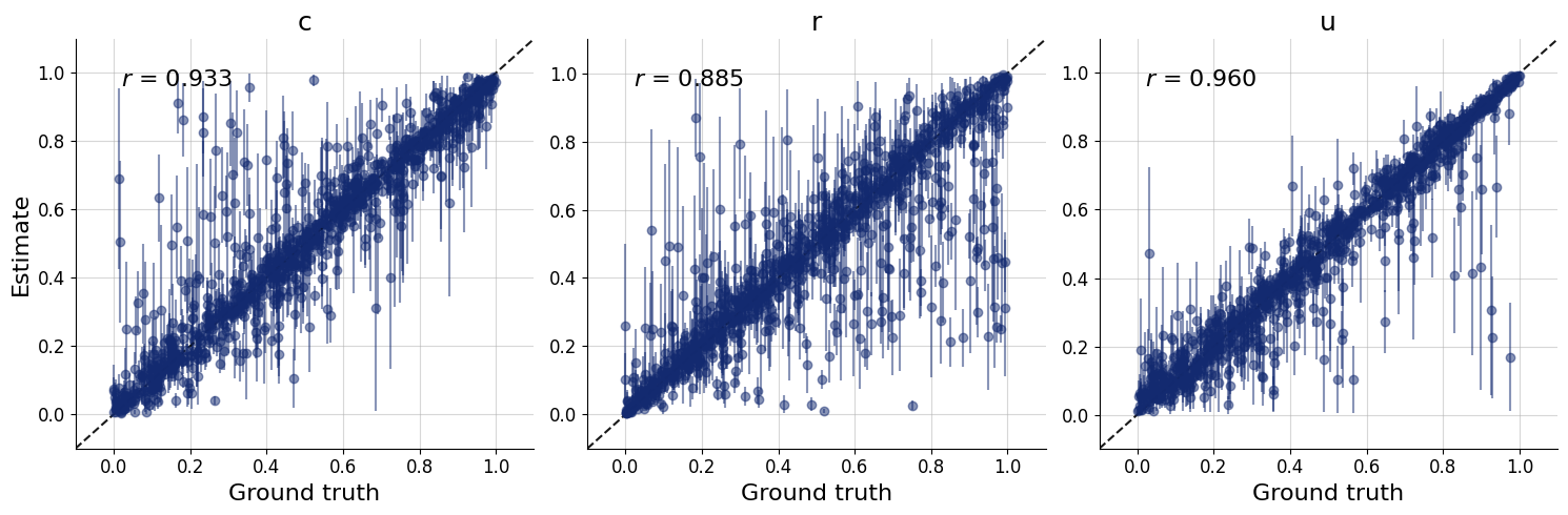
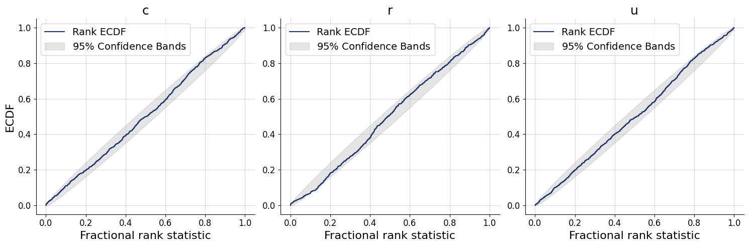
history=workflow.fit_online(epochs=20, num_batches_per_epoch=100, batch_size=256)

Validation

Code

test_data = simulator.sample(1000)
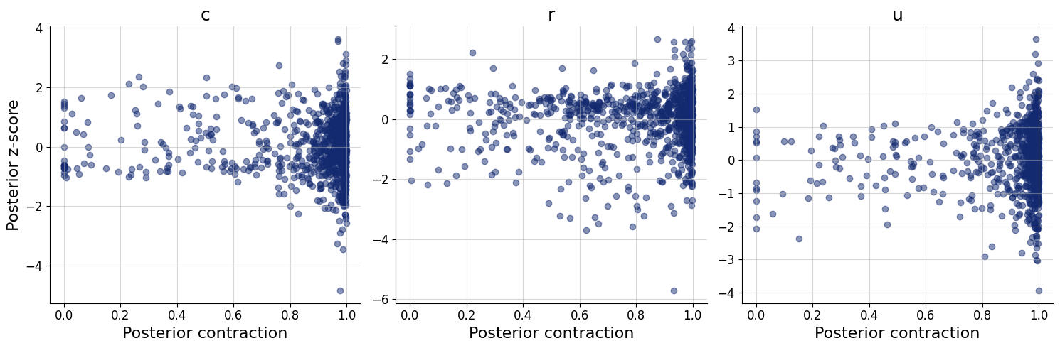
figs=workflow.plot_default_diagnostics(test_data=test_data, num_samples=500)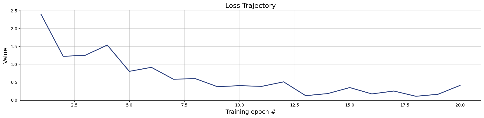

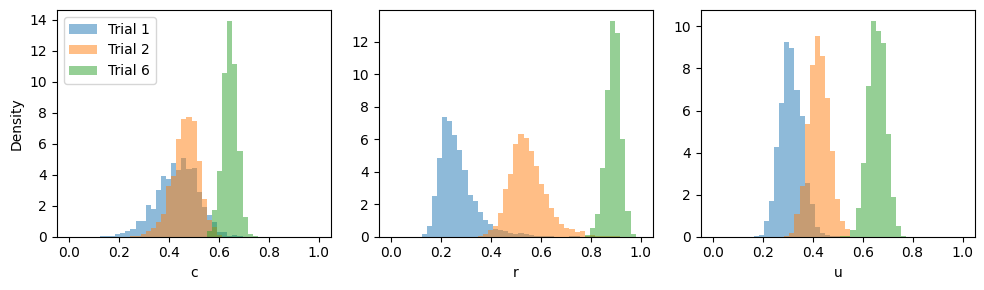
Inference

Here we will obtain the posterior distributions for trials 1, 2, and 6 from Riefer et al. (2002) as reported by Lee & Wagenmakers (2013).

Code

k = np.array([
    [45, 24, 97, 254],
    [106, 41, 107, 166],
    [243, 64, 65, 48]
])
inference_data = dict(k=k, n=np.sum(k, axis=-1)[..., np.newaxis])

Code

posterior_samples = workflow.sample(num_samples=2000, conditions=inference_data)

Code

plt.rcParams['figure.figsize'] = [10, 3]
fig, axes = plt.subplots(ncols=3)
axes = axes.flatten()
labels = ["Trial 1", "Trial 2", "Trial 6"]

for dat in range(len(labels)):
    for i, (par, samples)  in enumerate(posterior_samples.items()):
        axes[i].hist(samples[dat].flatten(), density=True, alpha=0.5, bins = np.linspace(0, 1, 50))
        axes[i].set_xlabel(par)
axes[0].legend(labels)
axes[0].set_ylabel("Density")


fig.tight_layout()

References

Lee, M. D., & Wagenmakers, E.-J. (2013). Bayesian Cognitive Modeling: A Practical Course. Cambridge University Press.

Riefer, D. M., Knapp, B. R., Batchelder, W. H., Bamber, D., & Manifold, V. (2002). Cognitive psychometrics: Assessing storage and retrieval deficits in special populations with multinomial processing tree models. Psychological Assessment, 14(2), 184.

Reuse

CC BY NC