Individual differences in the GCM

Author

Šimon Kucharský

Published

May 6, 2025

Code

import os

if "KERAS_BACKEND" not in os.environ:
    # set this to "torch", "tensorflow", or "jax"
    os.environ["KERAS_BACKEND"] = "jax"

import matplotlib.pyplot as plt
import numpy as np

import bayesflow as bf
import json

Here we will allow for individual differences between participants. The simplest way to start is to estimate the parameter values for each participant independently. Hence we estimate two parameters per participant. It may seem that we have to extend the model. However, since we assume that the participants are independent, we may as well simplify the model to assume data from a single participant only, and apply it to each participant in independently.

Data

We use the category learning data from the “Condensation B” condition from Kruschke (1993) as reported by Lee & Wagenmakers (2013).

Code

with open(os.path.join("data", "KruschkeData.json")) as f:
    data = json.load(f)

data.keys()

dict_keys(['a', 'd1', 'd2', 'n', 'nstim', 'nsubj', 'y'])

Simulator

We will reuse the prior and simulator from the first example of the GCM. The only difference is that we will remove the nsubj argument, and in so doing simplifying the simulation so that every data set contains data from a single participant.

Code

def prior():
    return dict(
        c = np.random.exponential(scale=1),
        w = np.random.uniform(low=0, high=1)
    )

def likelihood(c, w, n=data['n'], nstim=data['nstim'], d1=np.array(data['d1']), d2=np.array(data['d2']), a=np.array(data['a'])):
    b = 0.5

    s = np.exp( - c * (w * d1 + (1-w) * d2))

    r = np.zeros(nstim)

    for i in range(nstim):
        isA = a == 1
        isB = a != 1

        numerator = b * np.sum(s[i,isA])
        denominator = numerator + (1-b) * np.sum(s[i,isB])

        r[i] = numerator / denominator

    y = np.random.binomial(n=n, p=r, size=nstim)

    return dict(y=y)

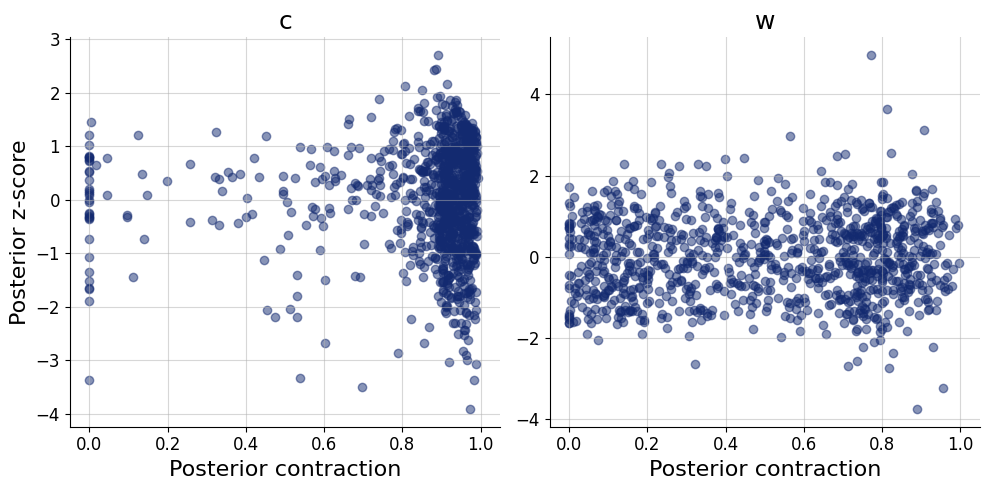
simulator = bf.make_simulator([prior, likelihood])

Approximator

We will use BasicWorkflow again. The task is to predict the posterior distribution of the parameters \(c\) and \(w\), given the observed data \(y\). Since \(y\) is of fixed size, we might not need a summary network.

Code

adapter = (bf.Adapter()
    .constrain("c", lower=0)
    .constrain("w", lower=0, upper=1)
    .concatenate(["c", "w"], into="inference_variables")
    .rename("y", "inference_conditions")
)

Code

workflow = bf.BasicWorkflow(
    simulator=simulator,
    adapter=adapter,
    inference_network=bf.networks.CouplingFlow(),
)

Training

Code

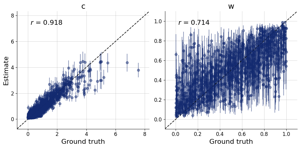
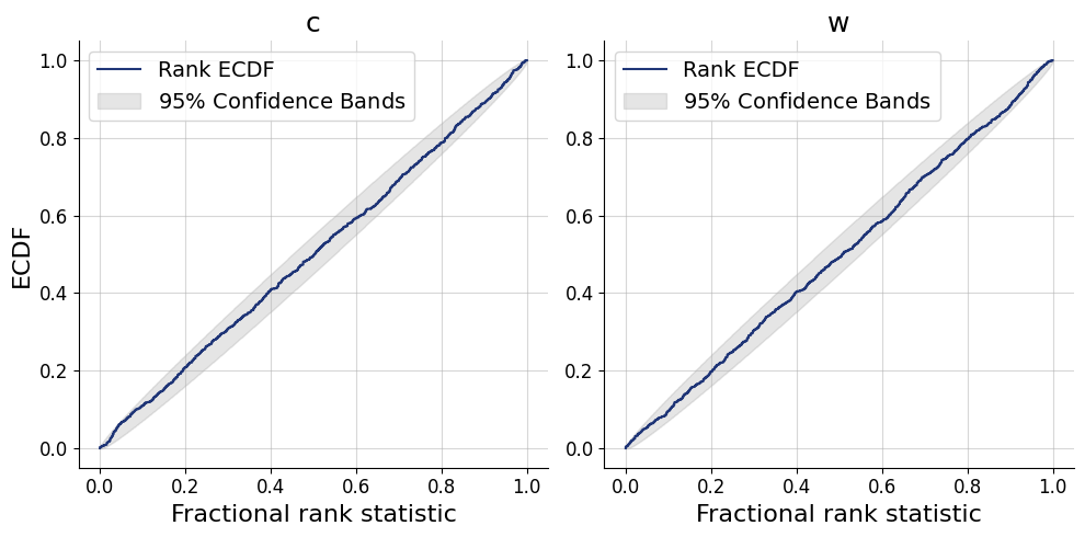
history=workflow.fit_online(epochs=50, batch_size=256)

Validation

Code

test_data = simulator.sample(1000)

Code

figs = workflow.plot_default_diagnostics(test_data=test_data, num_samples=500)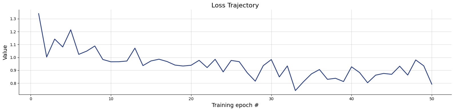

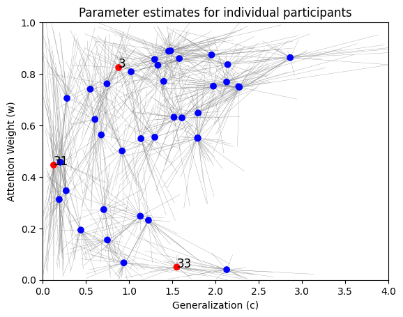
Inference

Now, we can use the approximator to obtain our posterior distributions of \(c\) and \(w\) for all 40 participants in the data set.

Code

inference_data = dict(y = np.array(data['y']).transpose())

inference_data['y'].shape

(40, 8)

Code

posterior_samples = workflow.sample(num_samples=2000, conditions=inference_data)

Code

posterior_means = {par: np.mean(samples, axis=1) for par, samples in posterior_samples.items()}

Code

highlight = [2, 30, 32]
cols = ["blue" if i not in highlight else "red" for i in range(data['nsubj'])]

plt.scatter(
    posterior_means['c'],
    posterior_means['w'], 
    color=cols, zorder=2)
for p in range(data['nsubj']):
    if p in highlight:
        plt.text(
            posterior_means['c'][p], 
            posterior_means['w'][p], 
            str(p+1), zorder=3, fontsize=12)
    for l in range(25):
        x = [posterior_means['c'][p], 
             posterior_samples['c'][p,l]
            ]
        y = [posterior_means['w'][p], 
             posterior_samples['w'][p,l]
            ]
        plt.plot(x, y, color="gray", linewidth=0.2, zorder=0)

plt.xlim(0, 4)
plt.xlabel("Generalization (c)")
plt.ylim(0, 1)
plt.ylabel("Attention Weight (w)")
f=plt.title("Parameter estimates for individual participants")

References

Kruschke, J. K. (1993). Human category learning: Implications for backpropagation models. Connection Science, 5(1), 3–36.

Lee, M. D., & Wagenmakers, E.-J. (2013). Bayesian Cognitive Modeling: A Practical Course. Cambridge University Press.

Reuse

CC BY NC