The GCM model

Author

Šimon Kucharský

Published

May 6, 2025

Code

import os

if "KERAS_BACKEND" not in os.environ:
    # set this to "torch", "tensorflow", or "jax"
    os.environ["KERAS_BACKEND"] = "jax"

import matplotlib.pyplot as plt
import numpy as np

import bayesflow as bf
import json

The basic model has three parameters - generalization (c), attention weight (w), and bias (b). In this example, we assume no bias between the categories, so b will be fixed to \(\frac{1}{2}\).

\[\begin{equation} \begin{aligned} c & \sim \text{Exponential}(0.5) \\ w & \sim \text{Uniform}(0, 1) \\ b & \leftarrow \frac{1}{2} \\ s_{ij} & \leftarrow \exp\left[- c \left(w d_{ij}^{(1)} + (1-w) d_{ij}^{(2)}\right)\right] \\ r_i & \leftarrow \frac{b \sum_j a_j s_{ij}}{b \sum_j a_j s_{ij} + (1-b) \sum_j (1-a_j) s_{ij}} \\ y_i & \sim \text{Binomial}(r_i, t) \end{aligned} \end{equation}\]

Data

We use the category learning data from the “Condensation B” condition reported by Kruschke (1993).

Code

with open(os.path.join("data", "KruschkeData.json")) as f:
    data = json.load(f)

data.keys()

dict_keys(['a', 'd1', 'd2', 'n', 'nstim', 'nsubj', 'y'])

The element y contains the array of responses \(y_{ik}\) for the trial \(i \in \{1, \dots, 8\}\) and participant \(k \in \{1, \dots, 40\}\).

Code

np.array(data['y']).shape

(8, 40)

d1 and d2 contain the physical distances between the 8 stimuli on the along the two dimensions, such that

\[\begin{equation} d_{ij}^{(k)} = | p_{ik} - p_{jk} | \end{equation}\]

The indicator vector a contains information whether the stimulus \(a_i\) is an element from Category A or an element from Category B.

Here we will assume that the design of the experiment (i.e., number of trials, number of stimuli, number of participants, nature of the stimuli) is fixed. That is, we will only amortize over the observation outcomes.

Simulator

Code

def prior():
    return dict(
        c = np.random.exponential(scale=1),
        w = np.random.uniform(low=0, high=1)
    )

def likelihood(c, w, n=data['n'], nstim=data['nstim'], nsubj=data['nsubj'], d1=np.array(data['d1']), d2=np.array(data['d2']), a=np.array(data['a'])):
    b = 0.5

    s = np.exp( - c * (w * d1 + (1-w) * d2))

    r = np.zeros((nsubj, nstim))

    for i in range(nstim):
        isA = a == 1
        isB = a != 1

        numerator = b * np.sum(s[i,isA])
        denominator = numerator + (1-b) * np.sum(s[i,isB])

        r[:, i] = numerator / denominator

    y = np.random.binomial(n=n, p=r, size=(nsubj, nstim))

    return dict(y=y)

simulator = bf.make_simulator([prior, likelihood])

Approximator

Code

adapter = (bf.Adapter()
    .constrain("c", lower=0)
    .constrain("w", lower=0, upper=1)
    .concatenate(["c", "w"], into="inference_variables")
    .rename("y", "summary_variables")
)

Code

workflow=bf.BasicWorkflow(
    simulator=simulator,
    adapter=adapter,
    inference_network=bf.networks.CouplingFlow(),
    summary_network=bf.networks.DeepSet(),
    initial_learning_rate=1e-3
)

Training

Code

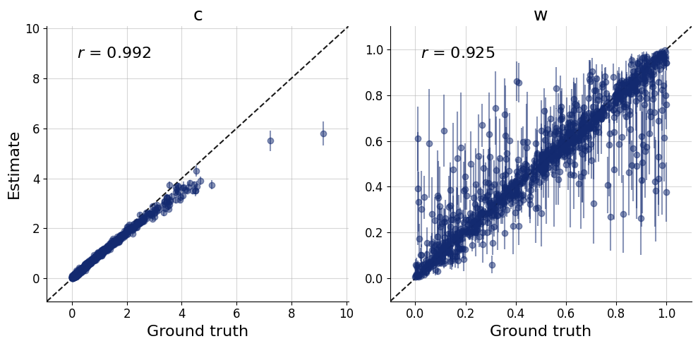
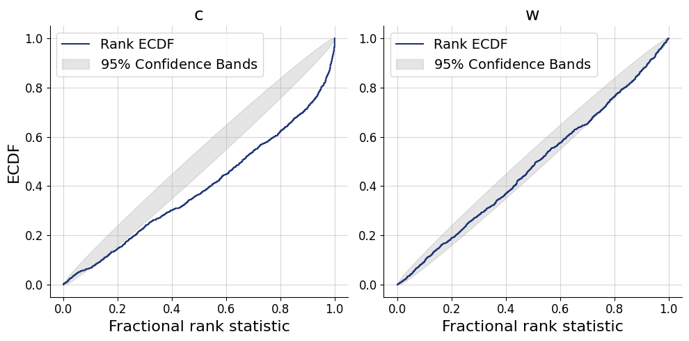
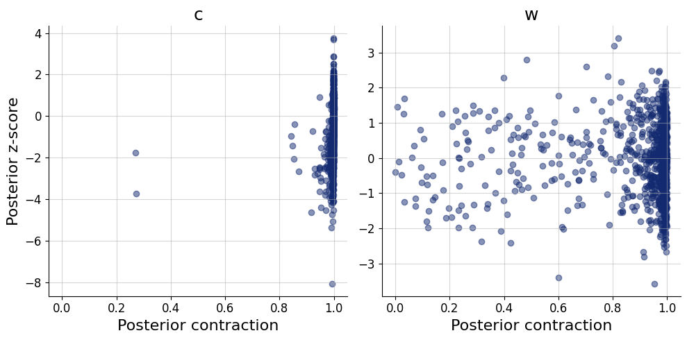
history=workflow.fit_online(batch_size=256)

Validation

Code

test_data = simulator.sample(1000)

Code

figs = workflow.plot_default_diagnostics(test_data=test_data, num_samples=500)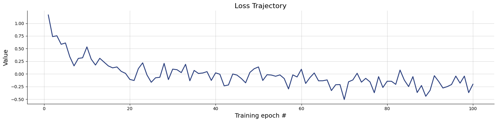

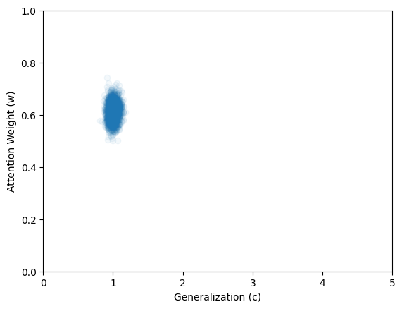
Inference

Here we apply the networks to the data from Kruschke (1993) as reported by Lee & Wagenmakers (2013). The quantity of interest is the joint posterior distribution of parameters \(c\) and \(w\).

Code

inference_data = dict(y = np.array(data['y']).transpose()[np.newaxis,...])

Code

posterior_samples = workflow.sample(num_samples=2000, conditions=inference_data)

Code

plt.scatter(
    x = posterior_samples['c'],
    y = posterior_samples['w'],
    alpha=0.05
)
plt.xlim([0, 5])
plt.ylim([0, 1])
plt.xlabel("Generalization (c)")
f=plt.ylabel("Attention Weight (w)")

References

Kruschke, J. K. (1993). Human category learning: Implications for backpropagation models. Connection Science, 5(1), 3–36.

Lee, M. D., & Wagenmakers, E.-J. (2013). Bayesian Cognitive Modeling: A Practical Course. Cambridge University Press.

Reuse

CC BY NC