Inferring a common rate

Author

Šimon Kucharský

Published

May 6, 2025

Code

import os

if "KERAS_BACKEND" not in os.environ:
    # set this to "torch", "tensorflow", or "jax"
    os.environ["KERAS_BACKEND"] = "jax"

import matplotlib.pyplot as plt
import numpy as np
import bayesflow as bf

INFO:bayesflow:Using backend 'jax'

In this section we will estimate a common binomial rate that produces two binomial processes according to the following model:

\[\begin{equation} \begin{aligned} k_1 & \sim \text{Binomial}(\theta, n_1) \\ k_2 & \sim \text{Binomial}(\theta, n_2) \\ \theta & \sim \text{Beta}(1, 1). \end{aligned} \end{equation}\]

Simulator

The individual components of the model are very similar to a combination of the previous two examples: Now we have one binomial proportion but two binomial outcomes.

Code

def context():
    return dict(n=np.random.randint(1, 101, size=2))

def prior():
    return dict(theta=np.random.beta(a=1, b=1))

def likelihood(n, theta):
    return dict(k=np.random.binomial(n=n, p=theta))

simulator=bf.make_simulator([context, prior, likelihood])

Approximator

Code

adapter = (
    bf.Adapter()
    .constrain("theta", lower=0, upper=1)
    .rename("theta", "inference_variables")
    .concatenate(["k", "n"], into="inference_conditions")
)

Code

workflow=bf.BasicWorkflow(
    simulator=simulator,
    adapter=adapter,
    inference_network=bf.networks.CouplingFlow()
)

Training

Code

history=workflow.fit_online(epochs=20, batch_size=512)

Validation

Code

test_data=simulator.sample(1000)
figs=workflow.plot_default_diagnostics(test_data=test_data, num_samples=500)

Inference

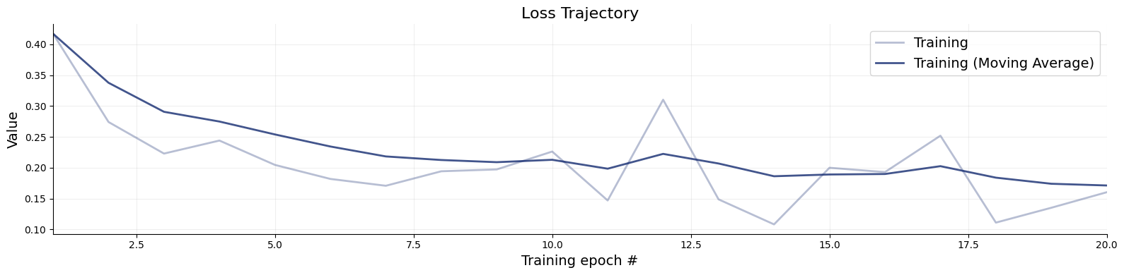
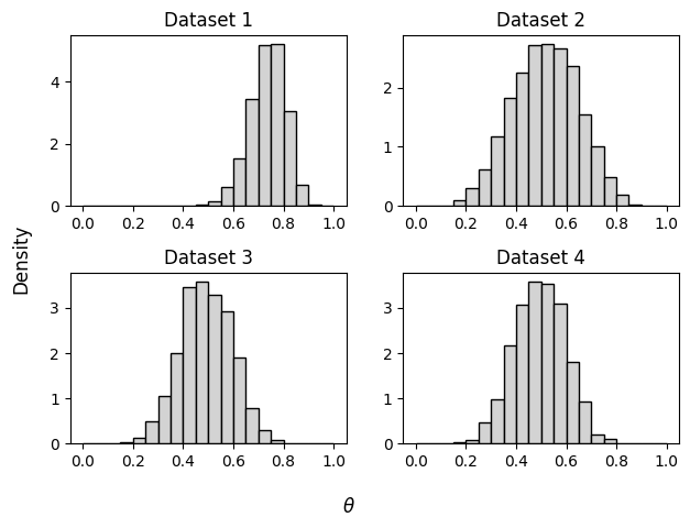
Now that we trained the network we can use it for inference. We are given four data sets by Lee & Wagenmakers (2013):

\(k_1 = 14\), \(k_2 = 16\), \(n_1 = n_2 = 20\)
\(k_1 = 0\), \(k_2 = 10\), \(n_1 = n_2 = 10\)
\(k_1 = 7\), \(k_2 = 3\), \(n_1 = n_2 = 10\)
\(k_1 = k_2 = 5\), \(n_1 = n_2 = 10\)

The advantage of BayesFlow is that we can obtain the samples for these three independent data sets at once. We simply define an array of data sets that are passed to the inference network.

Code

inference_data=dict(
    k = np.array([[14, 16], [0, 10], [7, 3], [5, 5]]),
    n = np.array([[20, 20], [10, 10], [10, 10], [10, 10]])
)

Code

samples=workflow.sample(num_samples=2000, conditions=inference_data)

Code

fig, axs = plt.subplots(nrows=2, ncols=2)
axs=axs.flatten()

for i, ax in enumerate(axs):
    ax.set_title("Dataset " + str(i + 1))
    ax.hist(samples["theta"][i], 
            density=True, color="lightgray", edgecolor="black", bins=np.arange(0, 1.05, 0.05))

fig.supxlabel(r"$\theta$")
fig.supylabel("Density")
fig.tight_layout()

References

Lee, M. D., & Wagenmakers, E.-J. (2013). Bayesian Cognitive Modeling: A Practical Course. Cambridge University Press.

Reuse

CC BY NC