Take the best model

Author

Šimon Kucharský

Published

May 6, 2025

Code

import os

if "KERAS_BACKEND" not in os.environ:
    # set this to "torch", "tensorflow", or "jax"
    os.environ["KERAS_BACKEND"] = "jax"

import matplotlib.pyplot as plt
import numpy as np

import bayesflow as bf
import json

\[\begin{equation} \begin{aligned} \gamma & \sim \text{Uniform}(0.5, 1) \\ y_{iq} & \sim \begin{cases} \text{Bernoulli}(\gamma) & \text{if } t_q = a \\ \text{Bernoulli}(1-\gamma) & \text{if } t_q = b \\ \text{Bernoulli}(0.5) & \text{otherwise}, \\ \end{cases} \end{aligned} \end{equation}\] where \(t_q\) is determined by the take the best decision rule defined below.

Data

Code

with open(os.path.join("data", "StopSearchData.json")) as f:
    data = json.load(f)

data.keys()

dict_keys(['m', 'nc', 'nq', 'ns', 'p', 'v', 'x', 'y'])

Simulator

First, we define the “take the best” (TTB) decision rule: For each question, we loop over its cues in order of their validity (the questions are already ordered in the data). As soon as a cue prefers decision ‘a’ or ‘b’, the decision is determined.

Code

def ttb(nq: int, nc: int, p: np.ndarray, m: np.ndarray):
    output = np.zeros(nq) # 0: guessing

    for q in range(nq):
        for c in range(nc):
            cue_a = m[p[q][0]-1][c]
            cue_b = m[p[q][1]-1][c]
            if cue_a > cue_b:
                output[q] = 1 # decision a
                break
            elif cue_a < cue_b:
                output[q] = 2 # decision b
                break

    return output.astype(int)

Applying the decision rule to the data produces the “decision a” for each question according to TTB: This is because the recorded data had been already recoded such that choice “a” always corresponds to the choice according to the TTB rule.

Code

decisions = ttb(data['nq'], data['nc'], data['p'], data['m'])
decisions

array([1, 1, 1, 1, 1, 1, 1, 1, 1, 1, 1, 1, 1, 1, 1, 1, 1, 1, 1, 1, 1, 1,
       1, 1, 1, 1, 1, 1, 1, 1])

Next, we can define the prior and a likelihood. The only source of alleatoric uncertainty in our simulator comes from the parameter \(\gamma\), which indicates the probability of responding “a” if the TTB decision rule indicates to respond “a”, and vice versa.

The shape of the resulting data is (number of participants, number of questions).

Code

def prior():
    return dict(gamma = np.random.uniform(low=0.5, high=1))
    

def likelihood(
        gamma: float, 
        ns: int = data['ns'],
        nq: int = data['nq'],
        ttb = decisions
        ):
    
    probs = np.array([0.5, gamma, 1-gamma])
    probs = probs[ttb][np.newaxis]
    probs = np.tile(probs, reps=[ns, 1])

    y = np.random.binomial(n=1, p=probs, size=(ns, nq))

    return dict(y=y)

simulator = bf.make_simulator([prior, likelihood])

Approximator

We will approximate the posterior of \(\gamma\), given the observed decisions \(y\).

Code

adapter = (bf.Adapter()
    .constrain("gamma", lower=0.5, upper=1)
    .rename("gamma", "inference_variables")
    .rename("y", "summary_variables")
)

Code

workflow = bf.BasicWorkflow(
    simulator=simulator,
    adapter=adapter,
    inference_network=bf.networks.CouplingFlow(),
    summary_network=bf.networks.DeepSet(),
    initial_learning_rate=1e-3
)

Training

Code

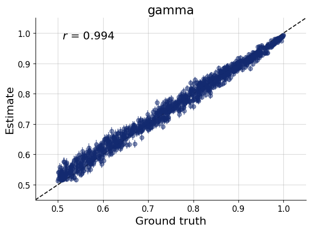
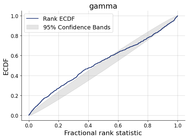
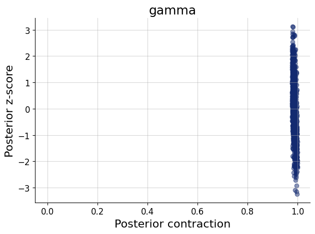
history = workflow.fit_online(epochs=50, num_batches_per_epoch=500, batch_size=512)

Validation

Code

test_data = simulator.sample(1000)

Code

figs=workflow.plot_default_diagnostics(test_data=test_data, num_samples=500)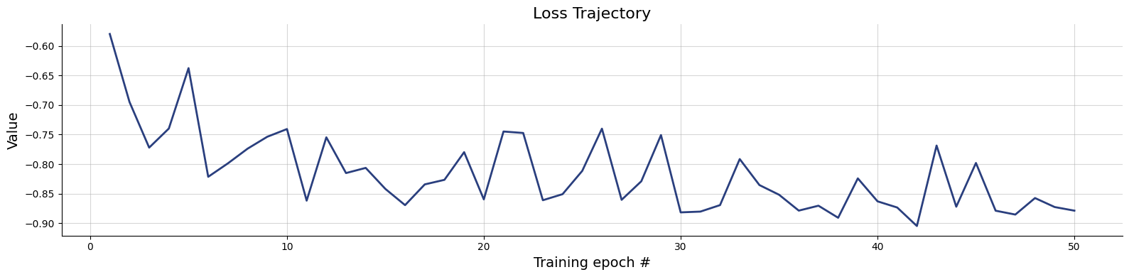

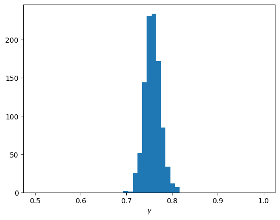
Inference

Now we can apply to the model to real data (Lee & Wagenmakers, 2013).

Code

inference_data = dict(y = np.array(data['y'])[np.newaxis])

Code

samples = workflow.sample(num_samples=1000, conditions=inference_data)

Code

f=plt.hist(samples['gamma'].flatten(), bins=np.linspace(0.5, 1, 50))
f=plt.xlabel(r"$\gamma$")

References

Lee, M. D., & Wagenmakers, E.-J. (2013). Bayesian Cognitive Modeling: A Practical Course. Cambridge University Press.

Reuse

CC BY NC