One-sample comparison

Author

Šimon Kucharský

Published

May 6, 2025

Code
import os

if "KERAS_BACKEND" not in os.environ:
    # set this to "torch", "tensorflow", or "jax"
    os.environ["KERAS_BACKEND"] = "jax"

import matplotlib.pyplot as plt
import numpy as np
import bayesflow as bf
import keras
INFO:bayesflow:Using backend 'jax'

\[\begin{equation} \begin{aligned} \mathcal{M_0}: \delta & = 0 \\ \mathcal{M_1}: \delta & \sim \text{Cauchy}(0, 1) \\[15pt] \sigma & \sim \text{HalfCauchy}(0, 1) \\ \mu & = \delta\sigma \\ x_i & \sim \text{Normal}(\mu, \sigma) \end{aligned} \end{equation}\]

Simulator

We need to define two simulator: one that represents the null hypothesis that \(\delta = 0\), and one that represents the alternative hypothesis that \(\delta \neq 0\). Then, we wrap them in a ModelComparisonSimulator, that will sample from either of them randomly.

We will also amortize over different sample sizes. Here we do this by randomly sampling values between 10 and 100. In the simulators, we will make sure that the output is always of length 100 (maximum sample size); the elements in the array whose index exceeds the actual sample size are filled with zeros. To make it easier for the networks to summarise such data, we will also create a binary indicator variable observed, which is one when the element in x is filled with an actual value, and zero otherwise.

Code
max_n=100
def context():
    return dict(n=np.random.randint(10, max_n))

def prior_nuisance():
    sigma = np.random.standard_cauchy()
    sigma = np.abs(sigma)
    return dict(sigma=sigma)

def prior_null():
    return dict(delta=0)

def prior_alternative():
    return dict(delta=np.random.standard_cauchy())

def likelihood(sigma, delta, n):
    mu = sigma * delta
    x = np.zeros(max_n)
    x[:n] = np.random.normal(loc=mu, scale=sigma, size=n)

    observed = np.zeros(max_n)
    observed[:n] = 1

    return dict(x=x, observed=observed)
Code
simulator_null = bf.make_simulator([context, prior_nuisance, prior_null, likelihood])
simulator_alt = bf.make_simulator([context, prior_nuisance, prior_alternative, likelihood])

simulator = bf.simulators.ModelComparisonSimulator([simulator_null, simulator_alt])

Approximator

The sample size is passed into the inference network directly, and the observations in x and the observed indicator are passed into a summary network first.

Code
adapter=(
    bf.Adapter()
    .as_set(["x", "observed"])
    .rename("n", "classifier_conditions")
    .concatenate(["x", "observed"], into="summary_variables")
    .drop(["delta","sigma"])
    )

Model comparison needs a classifier network to predict the posterior model probabilities. Here, we define a simple multi-layer perceptron to do this task.

Code
inference_network = keras.Sequential([
    keras.layers.Dense(32, activation="gelu")
    for _ in range(6)
])

Then we wrap everything together.

Code
approximator=bf.approximators.ModelComparisonApproximator(
    num_models=2,
    classifier_network=inference_network, 
    summary_network=bf.networks.DeepSet(
        summary_dim=4,
        mlp_widths_equivariant=(32, 32),
        mlp_widths_invariant_inner=(32, 32),
        mlp_widths_invariant_outer=(32, 32),
        mlp_widths_invariant_last=(32, 32)
    ),
    adapter=adapter
)

Training

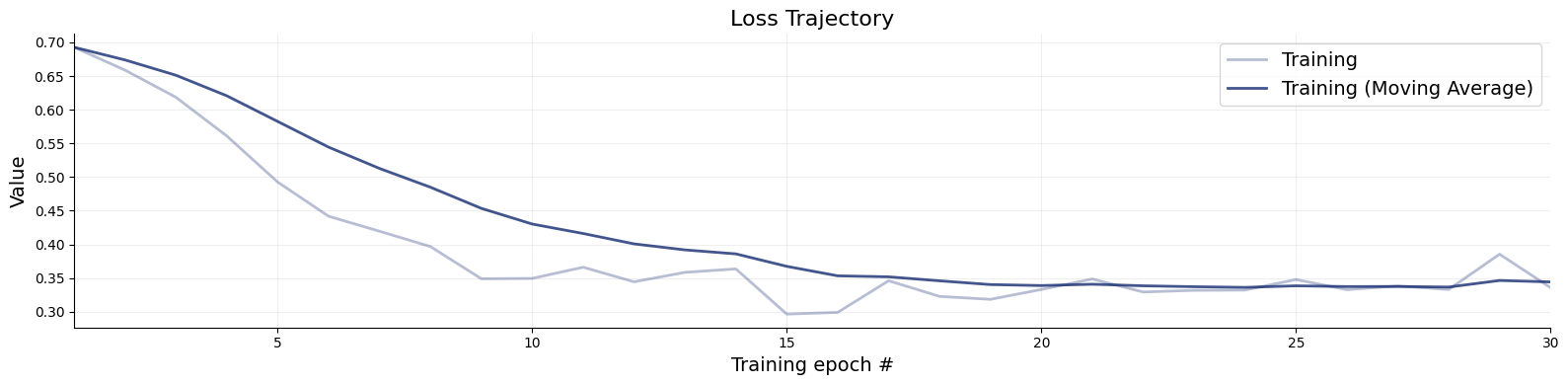
Here we will do offline traing. First, we will define the number of epochs, and the simulation budget (number of batches times the batch size). We also define an optimizer with a cosine decay schedule.

Code
epochs=30
batches=20
batch_size=512
schedule=keras.optimizers.schedules.CosineDecay(1e-4, decay_steps=epochs*batches)
optimizer=keras.optimizers.Adam(schedule)
approximator.compile(optimizer)

Now we can prepare our training dataset.

Code
train_data=simulator.sample(batches*batch_size)

train_data=bf.datasets.OfflineDataset(
    data=train_data, 
    batch_size=batch_size, 
    adapter=adapter)
Code
history=approximator.fit(
    dataset=train_data,
    epochs=epochs, 
    num_batches=batches, 
    batch_size=batch_size)
Code
f=bf.diagnostics.plots.loss(history=history)

Validation

Code
test_data=simulator.sample(1000)
Code
true_models = test_data["model_indices"]
pred_models = approximator.predict(conditions=test_data)
Code
f=bf.diagnostics.plots.mc_calibration(
    pred_models=pred_models,
    true_models=true_models,
    model_names=[r"$\mathcal{M}_0$",r"$\mathcal{M}_1$"],
)
INFO:matplotlib.mathtext:Substituting symbol M from STIXNonUnicode

Code
f=bf.diagnostics.plots.mc_confusion_matrix(
    pred_models=pred_models,
    true_models=true_models,
    model_names=[r"$\mathcal{M}_0$",r"$\mathcal{M}_1$"],
    normalize="true"
)
INFO:matplotlib.mathtext:Substituting symbol M from STIXNonUnicode

Inference

Code
winter=np.array([-0.05,0.41,0.17,-0.13,0.00,-0.05,0.00,0.17,0.29,0.04,0.21,0.08,0.37,0.17,0.08,-0.04,-0.04,0.04,-0.13,-0.12,0.04,0.21,0.17,
       0.17,0.17,0.33,0.04,0.04,0.04,0.00,0.21,0.13,0.25,-0.05,0.29,0.42,-0.05,0.12,0.04,0.25,0.12])
summer=np.array([0.00,0.38,-0.12,0.12,0.25,0.12,0.13,0.37,0.00,0.50,0.00,0.00,-0.13,-0.37,-0.25,-0.12,0.50,0.25,0.13,0.25,0.25,0.38,0.25,0.12,
      0.00,0.00,0.00,0.00,0.25,0.13,-0.25,-0.38,-0.13,-0.25,0.00,0.00,-0.12,0.25,0.00,0.50,0.00])
n = len(winter)

x = np.zeros(max_n)
x[:n] = winter-summer
observed = np.zeros(max_n)
observed[:n] = 1

inference_data = dict(
    n = np.array([[n]]),
    x = x[np.newaxis],
    observed = observed[np.newaxis]
)
Code
pred_models = approximator.predict(conditions=inference_data)[0]
Code
pred_models[0]/pred_models[1]
4.933184

The Bayes Factor is about 5 in favour in the null model.

References

Lee, M. D., & Wagenmakers, E.-J. (2013). Bayesian Cognitive Modeling: A Practical Course. Cambridge University Press.

Reuse