No individual differences

Author

Šimon Kucharský

Published

May 6, 2025

Code

import os

if "KERAS_BACKEND" not in os.environ:
    # set this to "torch", "tensorflow", or "jax"
    os.environ["KERAS_BACKEND"] = "jax"

import matplotlib.pyplot as plt
import numpy as np
import bayesflow as bf

INFO:bayesflow:Using backend 'jax'

\[\begin{equation} \begin{aligned} \alpha & \sim \text{Beta}(1, 1) \\ \beta & \sim \text{Beta}(1, 1) \\ \theta_i' & \leftarrow \exp(-\alpha t_i) + \beta \\ \theta_i & \leftarrow \begin{cases} 0 & \text{if } \theta_i' < 0 \\ 1 & \text{if } \theta_i' > 1 \\ \theta_i' & \text{otherwise} \end{cases} \\ k_i & \sim \text{Binomial}(\theta_i, 18) \end{aligned} \end{equation}\]

Simulator

Code

def prior():
    alpha = np.random.beta(a=1, b=1)
    beta = np.random.beta(a=1, b=1)
    return dict(alpha=alpha, beta=beta)

def likelihood(alpha, beta, t=np.array([1, 2, 4, 7, 12, 21, 35, 59, 99])):
    theta = np.exp(-alpha*t) + beta
    theta = np.clip(theta, a_min=0, a_max=1)

    k = np.random.binomial(n=18, p=theta, size=(3, len(theta)))
    return dict(k=k)

simulator = bf.make_simulator([prior, likelihood])

Approximator

Code

adapter = (
    bf.Adapter()
    .constrain(["alpha", "beta"], lower=0, upper=1)
    .concatenate(["alpha", "beta"], into="inference_variables")
    .rename("k", "summary_variables")
    )

Code

workflow = bf.BasicWorkflow(
    simulator=simulator,
    adapter=adapter,
    inference_network=bf.networks.CouplingFlow(),
    summary_network=bf.networks.DeepSet(),
    initial_learning_rate=1e-3
)

Training

Code

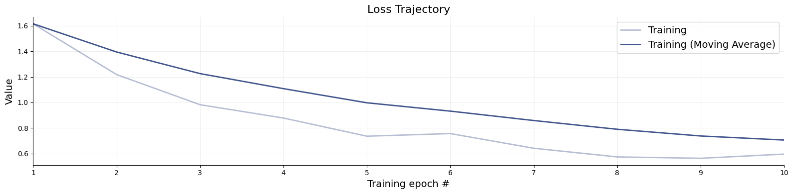
history=workflow.fit_online(epochs=10, num_batches_per_epoch=100, batch_size=1024)

Code

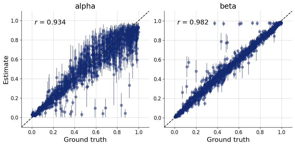
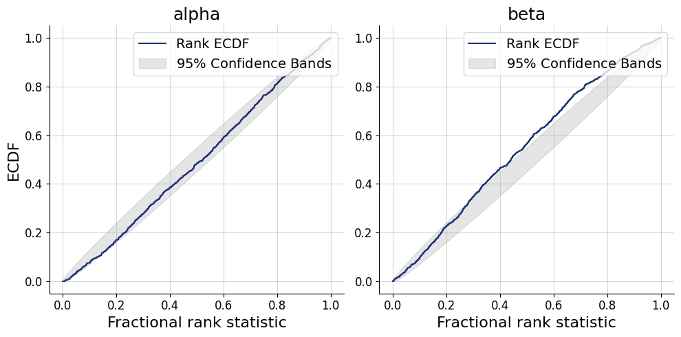
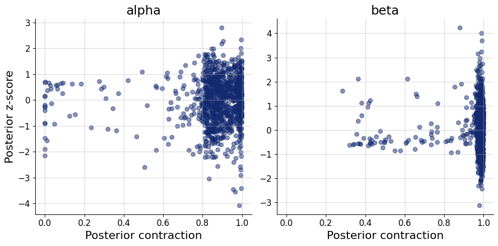
test_data = simulator.sample(1000)
figs = workflow.plot_default_diagnostics(test_data=test_data, num_samples=500)

Inference

We use the data from three participants by Rubin et al. (1999) as reported by Lee & Wagenmakers (2013).

Code

k = [[18, 18, 16, 13, 9, 6, 4, 4, 4],
     [17, 13,  9,  6, 4, 4, 4, 4, 4],
     [14, 10,  6,  4, 4, 4, 4, 4, 4]]

inference_data = dict(k=np.array(k)[np.newaxis])

Code

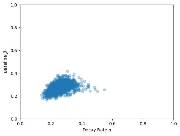
samples=workflow.sample(num_samples=2000, conditions=inference_data)

Code

plt.scatter(
    x=samples["alpha"], 
    y=samples["beta"], 
    alpha=0.3)
plt.xlim([0, 1])
plt.ylim([0, 1])
plt.xlabel("Decay Rate $\\alpha$")
plt.ylabel("Baseline $\\beta$")
None

References

Lee, M. D., & Wagenmakers, E.-J. (2013). Bayesian Cognitive Modeling: A Practical Course. Cambridge University Press.

Rubin, D. C., Hinton, S., & Wenzel, A. (1999). The precise time course of retention. Journal of Experimental Psychology: Learning, Memory, and Cognition, 25(5), 1161.

Reuse

CC BY NC