Equality of proportions

Author

Šimon Kucharský

Published

May 6, 2025

Code

import os

if "KERAS_BACKEND" not in os.environ:
    # set this to "torch", "tensorflow", or "jax"
    os.environ["KERAS_BACKEND"] = "jax"

import matplotlib.pyplot as plt
import numpy as np
import bayesflow as bf
import keras

Here we will compare two models. The null model assumes that proportion is the same for two binomial data sets

\[\begin{equation} \begin{aligned} s_1 & \sim \text{Binomial}(\theta_1, n_1) \\ s_2 & \sim \text{Binomial}(\theta_1, n_2) \\ \theta_1 & \sim \text{Beta}(1, 1), \end{aligned} \end{equation}\] whereas the alternative model assumes that the two groups are associated with different binomial rates:

\[\begin{equation} \begin{aligned} s_1 & \sim \text{Binomial}(\theta_1, n_1) \\ s_2 & \sim \text{Binomial}(\theta_1, n_2) \\ \theta_1 & \sim \text{Beta}(1, 1) \\ \theta_2 & \sim \text{Beta}(1, 1). \end{aligned} \end{equation}\]

Simulator

We will also amortize over different sample sizes for each group.

Code

def context():
    n = np.random.randint(1000, 10_000, size=2)
    return dict(n = n)

def prior_null():
    theta = np.random.beta(a=1, b=1)
    return dict(theta = np.array([theta, theta]))

def prior_alternative():
    theta = np.random.beta(a=1, b=1, size=2)
    return dict(theta = theta)

def likelihood(theta, n):
    s = np.random.binomial(n=n, p=theta)
    return dict(s=s)

simulator_null = bf.make_simulator([context, prior_null, likelihood])
simulator_alternative = bf.make_simulator([context, prior_alternative, likelihood])
simulator = bf.simulators.ModelComparisonSimulator(
    simulators=[simulator_null, simulator_alternative], 
    use_mixed_batches=True)

Approximator

Code

adapter = (
    bf.Adapter()
    .concatenate(['n', 's'], into="classifier_conditions")
    .drop('theta')
    )

Code

classifier_network = keras.Sequential([
    keras.layers.Dense(32, activation="gelu")
    for _ in range(8)
])
approximator = bf.approximators.ModelComparisonApproximator(
    num_models=2, 
    classifier_network=classifier_network, 
    adapter=adapter)

Training

Code

epochs = 30
num_batches = 100
batch_size = 512

learning_rate = keras.optimizers.schedules.CosineDecay(5e-4, decay_steps=epochs*num_batches)
optimizer = keras.optimizers.Adam(learning_rate=learning_rate, clipnorm=1.0)
approximator.compile(optimizer=optimizer)

Code

history = approximator.fit(
    epochs=epochs,
    num_batches=num_batches,
    batch_size=batch_size,
    simulator=simulator,
    adapter=adapter
)

Code

f=bf.diagnostics.plots.loss(history=history)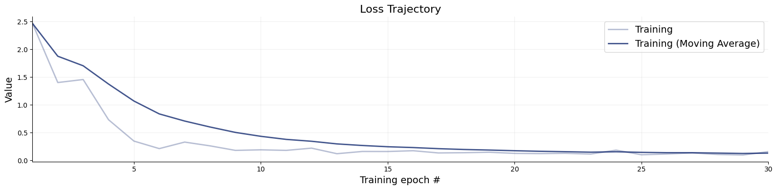

Validation

Code

test_data=simulator.sample(5_000)

Code

true_models=test_data["model_indices"]
pred_models=approximator.predict(conditions=test_data)

Code

f=bf.diagnostics.plots.mc_calibration(
    pred_models=pred_models,
    true_models=true_models,
    model_names=[r"$\mathcal{M}_0$",r"$\mathcal{M}_1$"],
)

INFO:matplotlib.mathtext:Substituting symbol M from STIXNonUnicode
INFO:matplotlib.mathtext:Substituting symbol M from STIXNonUnicode
INFO:matplotlib.mathtext:Substituting symbol M from STIXNonUnicode
INFO:matplotlib.mathtext:Substituting symbol M from STIXNonUnicode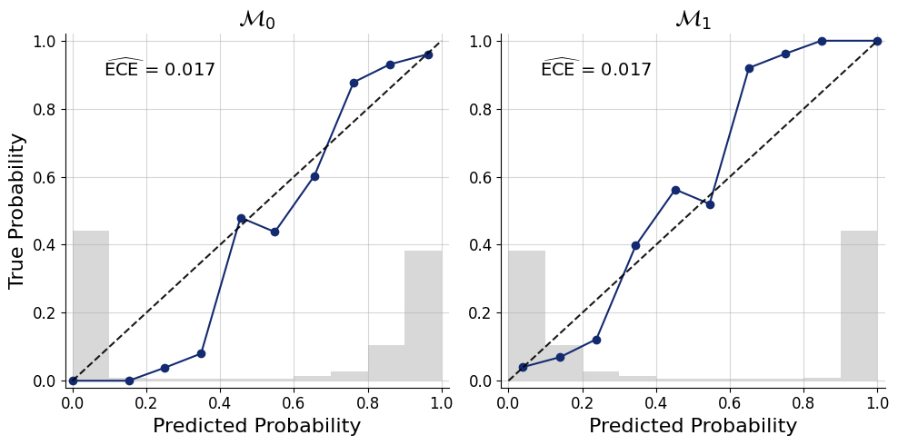

Code

f=bf.diagnostics.plots.mc_confusion_matrix(
    pred_models=pred_models,
    true_models=true_models,
    model_names=[r"$\mathcal{M}_0$",r"$\mathcal{M}_1$"],
    normalize="true"
)

INFO:matplotlib.mathtext:Substituting symbol M from STIXNonUnicode
INFO:matplotlib.mathtext:Substituting symbol M from STIXNonUnicode
INFO:matplotlib.mathtext:Substituting symbol M from STIXNonUnicode
INFO:matplotlib.mathtext:Substituting symbol M from STIXNonUnicode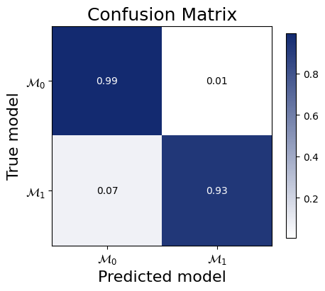

Inference

Code

inference_data = dict(n = np.array([[5416, 9072]]), s = np.array([[424, 777]]))

Code

pred_models = approximator.predict(conditions=inference_data)[0]
pred_models

array([0.9855641 , 0.01443596], dtype=float32)

Code

pred_models[1]/pred_models[0]

0.014647411

References

Lee, M. D., & Wagenmakers, E.-J. (2013). Bayesian Cognitive Modeling: A Practical Course. Cambridge University Press.

Reuse

CC BY NC