Full individual differences

import os

if "KERAS_BACKEND" not in os.environ:
    # set this to "torch", "tensorflow", or "jax"
    os.environ["KERAS_BACKEND"] = "jax"

import matplotlib.pyplot as plt
import numpy as np
import bayesflow as bf

import matplotlib.patches as mpatches

The model is the same as in the previous example, though can be simplified since we fit the model for each participant separately.

\[\begin{equation} \begin{aligned} \alpha & \sim \text{Beta}(1, 1) \\ \beta & \sim \text{Beta}(1, 1) \\ \theta_i' & \leftarrow \exp(-\alpha t_i) + \beta \\ \theta_i & \leftarrow \begin{cases} 0 & \text{if } \theta_i' < 0 \\ 1 & \text{if } \theta_i' > 1 \\ \theta_i' & \text{otherwise} \end{cases} \\ k_i & \sim \text{Binomial}(\theta_i, 18) \end{aligned} \end{equation}\]

Simulator

def prior():
    alpha = np.random.beta(a=1, b=1)
    beta = np.random.beta(a=1, b=1)
    return dict(alpha=alpha, beta=beta)

def likelihood(alpha, beta, t=np.array([1, 2, 4, 7, 12, 21, 35, 59, 99])):
    theta = np.exp(-alpha*t) + beta
    theta = np.clip(theta, a_min=0, a_max=1)

    k = np.random.binomial(n=18, p=theta)
    return dict(k=k)

simulator = bf.make_simulator([prior, likelihood])

Approximator

We will use the values of \(k\) to approximate the posterior distribution of \(\alpha\) and \(\beta\).

adapter = (
    bf.Adapter()
    .constrain(["alpha", "beta"], lower=0, upper=1)
    .concatenate(["alpha", "beta"], into="inference_variables")
    .rename("k", "inference_conditions")
    )

workflow = bf.BasicWorkflow(
    simulator=simulator,
    adapter=adapter,
    inference_network=bf.networks.CouplingFlow()
)

Training

history=workflow.fit_online(epochs=10, num_batches_per_epoch=100, batch_size=256)

Validation

test_data = simulator.sample(1000)
figs = workflow.plot_default_diagnostics(test_data=test_data, num_samples=500)

Inference

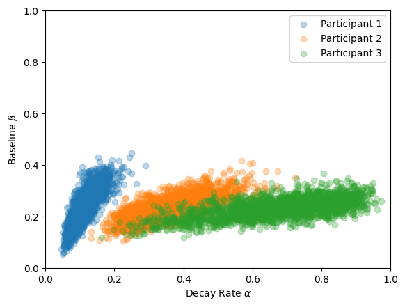
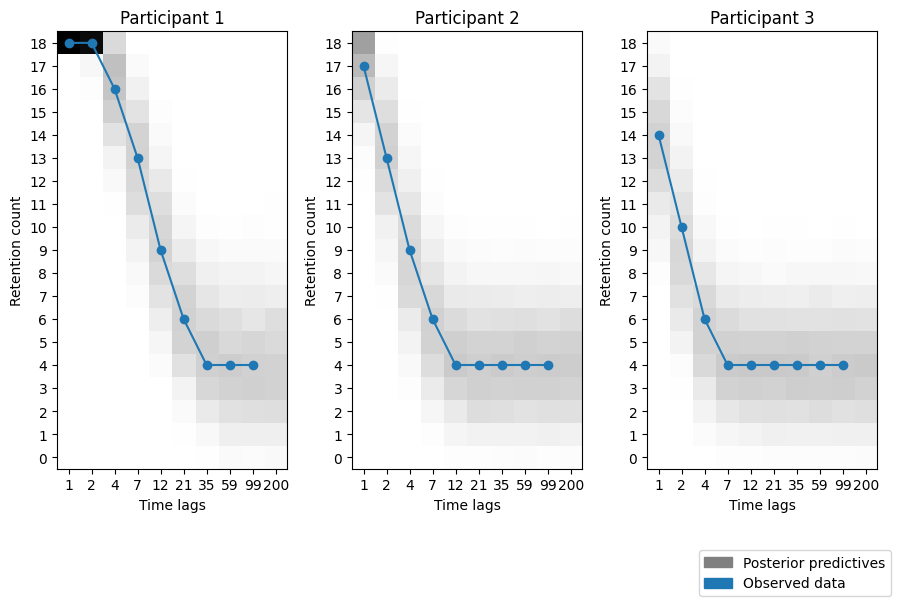
We use the data from three participants by Rubin et al. (1999) as reported by Lee & Wagenmakers (2013). We estimate the three posteriors simultaneously for all data sets (participants).

k = [[18, 18, 16, 13, 9, 6, 4, 4, 4],
     [17, 13,  9,  6, 4, 4, 4, 4, 4],
     [14, 10,  6,  4, 4, 4, 4, 4, 4]]

inference_data = dict(k=np.array(k))

samples=workflow.sample(num_samples=2000, conditions=inference_data)

for i in range(3):
    plt.scatter(
        x=samples["alpha"][i,:,0], 
        y=samples["beta"][i,:,0], 
        label="Participant "+str(i+1), 
        alpha=0.3)
plt.xlim([0, 1])
plt.ylim([0, 1])
plt.xlabel("Decay Rate $\\alpha$")
plt.ylabel("Baseline $\\beta$")
plt.legend()

Now we compute posterior predictives and plot them against the observed data.

k_pred = np.zeros((3, 2000, 10))

for p in range(3):
    for s in range(2000):
        k_pred[p, s, :] = likelihood(
            alpha=samples["alpha"][p, s, 0],
            beta=samples["beta"][p, s, 0],
            t=np.array([1, 2, 4, 7, 12, 21, 35, 59, 99, 200])
        )["k"]

# Bin the data and compute the relative frequencies for each possible count from 0 to 18.
hist = np.zeros((3, 19, 10))

for p in range(3):
    for t in range(10):
        hist[p, :, t] = np.histogram(k_pred[p, :, t], bins=19, range=[0, 19], density=True)[0]

fig, axs = plt.subplots(ncols=3, figsize=(9, 7))

for i, ax in enumerate(axs):
    ax.set_title("Participant " + str(i+1))
    ax.imshow(1-hist[i], 'gray', origin="lower", vmin=0, vmax=1)
    ax.set_xticks(range(10), labels=[1, 2, 4, 7, 12, 21, 35, 59, 99, 200])
    ax.set_xlabel("Time lags")
    ax.set_yticks(range(19))
    ax.set_ylabel("Retention count")
    ax.plot(range(9), inference_data["k"][i])
    ax.scatter(range(9), inference_data["k"][i])

custom_legend = [mpatches.Patch(color='gray', label='Posterior predictives'),
                 mpatches.Patch(color='#1f77b4', label='Observed data')]

fig.legend(handles=custom_legend, loc="lower right")
fig.tight_layout()

References

Lee, M. D., & Wagenmakers, E.-J. (2013). Bayesian Cognitive Modeling: A Practical Course. Cambridge University Press.

Rubin, D. C., Hinton, S., & Wenzel, A. (1999). The precise time course of retention. Journal of Experimental Psychology: Learning, Memory, and Cognition, 25(5), 1161.