Pearson correlation

Author

Šimon Kucharský

Published

May 6, 2025

Code

import os
if "KERAS_BACKEND" not in os.environ:
    # set this to "torch", "tensorflow", or "jax"
    os.environ["KERAS_BACKEND"] = "jax"

import numpy as np
import bayesflow as bf
import matplotlib.pyplot as plt

In this example we will estimate the population Pearson’s correlation \(\rho\). Although we could specify the full bivariate normal model as is the case if we want to estimate correlations in JAGS and similar, we do not have to. Instead, we will focus only on the parameter of interest, the correlation coefficient \(\rho\), and completely circumvent the necessity of estimating the means and variances of the two variables. Conceptually, our model is

\[\begin{equation} \begin{aligned} \rho & \sim \text{Uniform}(-1, 1) \\ \mathbb{y} & \sim \text{MvGaussian}\left((0, 0), \begin{bmatrix} 1 & \rho \\ \rho & 1\end{bmatrix} \right) \\ r & \leftarrow \text{cor}(\mathbb{y}), \end{aligned} \end{equation}\] where \(\text{cor}\) is just a function that takes a \(n \times 2\) matrix and returns the Pearson’s product moment correlation coefficient of the two columns.

Here, the parameter of interest is \(\rho\), and the data is summarised by \(r\) and \(n\). Therefore our inference will be invariant to the location and scaling of the variables by construction.

Simulator

Note that because the data is summarised by the pair \(r\) and \(n\), we can also vary \(n\) so that the model can make inferences on data from different sample sizes. We achieve this by specifying a context that will vary \(n\) for each simulation. Here we vary \(n\) between 3 and 100.

Code

def context():
    return dict(n=np.random.randint(3, 101))

def prior():
    return dict(rho=np.random.uniform(low=-1, high=1))

def likelihood(n, rho):
    y = np.random.multivariate_normal(mean=[0, 0], cov=[[1, rho], [rho, 1]], size = n)
    r = np.corrcoef(y[:,0], y[:,1])[0,1]
    return dict(r=r)

simulator = bf.make_simulator([context, prior, likelihood])

Approximator

Code

adapter=(
    bf.Adapter()
    .constrain("rho", lower=-1, upper=1)
    .rename("rho", "inference_variables")
    .concatenate(["n", "r"], into="inference_conditions")
)

Code

workflow=bf.BasicWorkflow(
    simulator=simulator,
    adapter=adapter,
    inference_network=bf.networks.CouplingFlow()
)

Training

Code

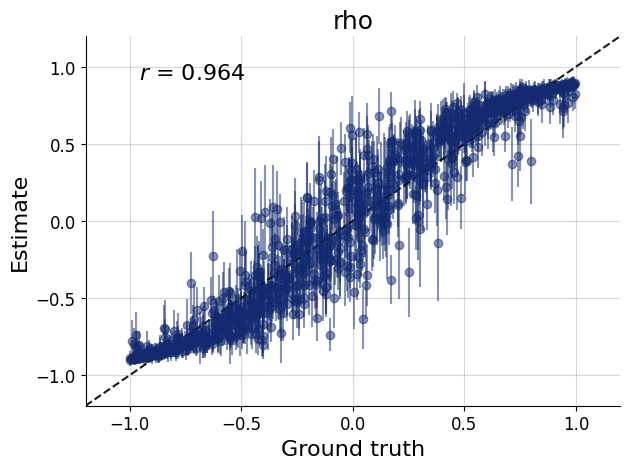
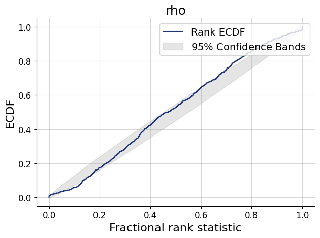
history=workflow.fit_online(epochs=20, batch_size=256)

Validation

Code

test_data=simulator.sample(1000)
figs=workflow.plot_default_diagnostics(test_data=test_data, num_samples=500)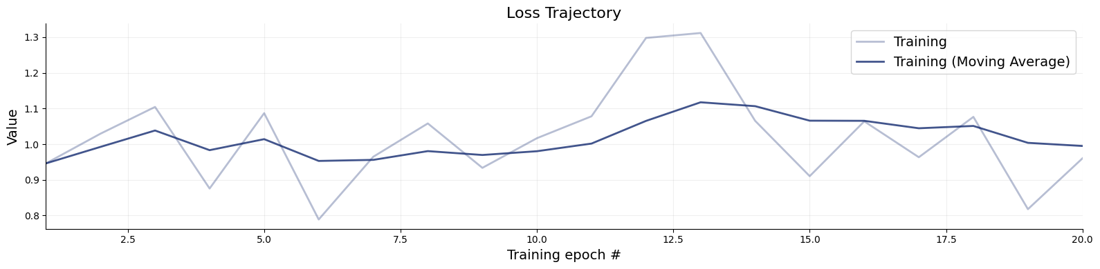

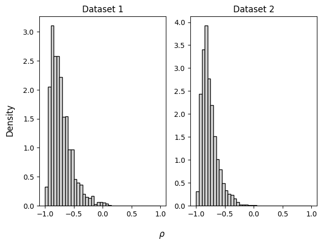
Inference

Now we can estimate the parameter \(\rho\) from data. We are provided two synthetic data sets (Lee & Wagenmakers, 2013), both of which result with the same Pearson correlation, but with a different sample size.

The advantage of BayesFlow is that once we have trained the networks we can very easily apply them to multiple data sets at the same time - simply pass them to the amortizer in an array.

Code

# summary statistics of data set 1: r = -0.8109671, n = 11
# summary statistics of data set 2: r = -0.8109671, n = 22
inference_data = dict(
    n = np.array([[11], [22]]),
    r = np.array([[-0.8109671], [-0.8109671]]))

Code

samples = workflow.sample(num_samples=2000, conditions=inference_data)

Code

fig, axs = plt.subplots(ncols=2)

for i, ax in enumerate(axs):
    ax.set_title("Dataset " + str(i + 1))
    ax.hist(samples["rho"][i], 
            density=True, color="lightgray", edgecolor="black", bins=np.arange(-1, 1.05, 0.05))

fig.supxlabel(r"$\rho$")
fig.supylabel("Density")
fig.tight_layout()

References

Lee, M. D., & Wagenmakers, E.-J. (2013). Bayesian Cognitive Modeling: A Practical Course. Cambridge University Press.

Reuse

CC BY NC