The BART model

Author

Šimon Kucharský

Published

May 6, 2025

Code

import os

if "KERAS_BACKEND" not in os.environ:
    # set this to "torch", "tensorflow", or "jax"
    os.environ["KERAS_BACKEND"] = "jax"

import matplotlib.pyplot as plt
import numpy as np
import bayesflow as bf

INFO:bayesflow:Using backend 'jax'

\[\begin{equation} \begin{aligned} \gamma & \sim \text{Exponential}(1) \\ \beta & \sim \text{Exponential}(1) \\ \omega & \leftarrow - \frac{\gamma}{\log(1-p)} \\ \theta_{jk} & \leftarrow \frac{1}{1 + \exp\left(\beta(k-\omega)\right)} \\ d_{jk} & \sim \text{Bernoulli}(\theta_{jk}) \end{aligned} \end{equation}\]

Simulator

Code

def prior():
    return dict(
        gamma = np.random.exponential(scale=1),
        beta = np.random.exponential(scale=1)
    )

def likelihood(gamma, beta, n_trials=90, p=0.15):
    omega = - gamma / np.log1p(-p)

    d = np.zeros(n_trials)

    for i in range(n_trials):
        n_pumps = 0

        while True: 
            theta = 1 / (1 + np.exp(beta * (n_pumps + 1 - omega)))

            pump = np.random.binomial(n=1, p=theta)
            if not pump:
                break

            n_pumps += 1

            bust = np.random.binomial(n=1, p=p)
            if bust:
                break
        
        d[i] = n_pumps
    
    return dict(d = d)

simulator = bf.make_simulator([prior, likelihood])

Approximator

We will use the BasicWorkflow to train an approximator that consists of an affine coupling flow inference network and a deep set summary network. The task is to infer the posterior distrobutions of \(\gamma\) and \(\delta\), given the observed decisions to pump the baloon (\(d\)) in each of the 90 trials.

Code

adapter = (bf.Adapter()
    .as_set("d")
    .constrain(["gamma", "beta"], lower=0)
    .standardize(["gamma", "beta"])
    .concatenate(["gamma", "beta"], into="inference_variables")
    .rename("d", "summary_variables")
)

Code

workflow = bf.BasicWorkflow(
    simulator=simulator,
    adapter=adapter,
    inference_network=bf.networks.CouplingFlow(),
    summary_network=bf.networks.DeepSet(),
    initial_learning_rate=1e-3
)

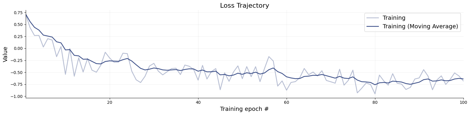
Training

Code

history=workflow.fit_online(epochs=100, num_batches_per_epoch=200, batch_size=128)

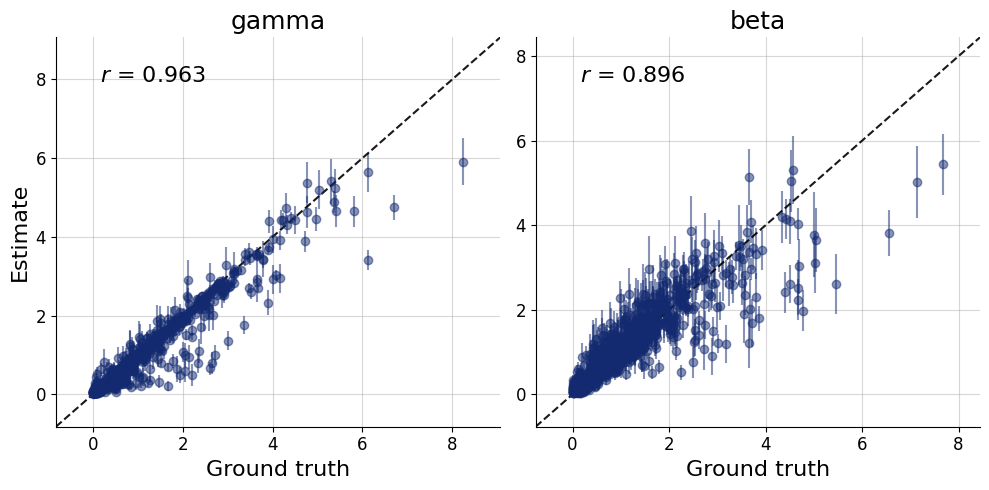
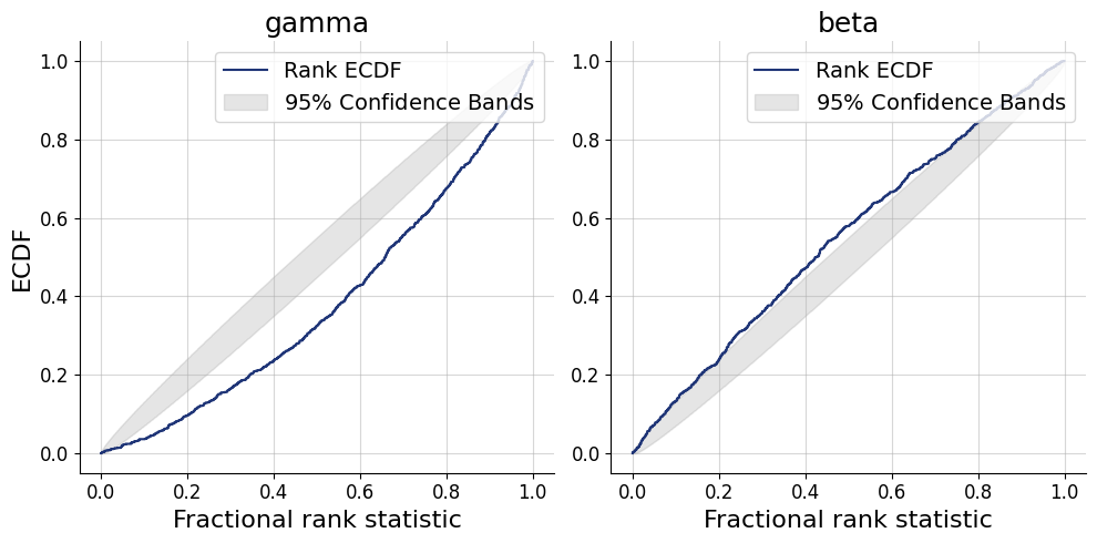
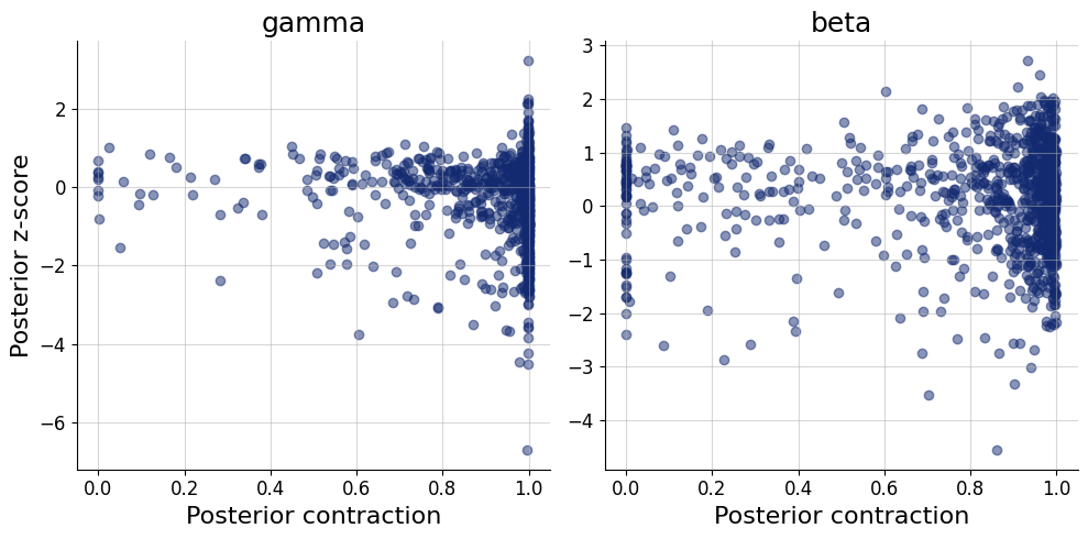
Validation

Code

test_data=simulator.sample(1000)

Code

figs=workflow.plot_default_diagnostics(test_data=test_data, num_samples=500)

Inference

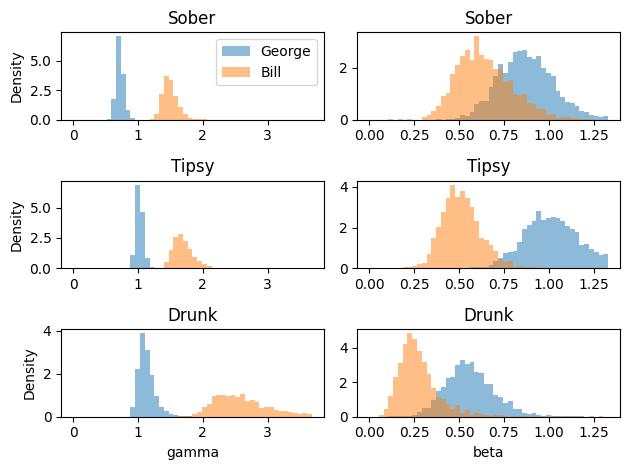
Here we will fit the model to two participants (George and Bill), each under three different conditions (Sober, Tipsy, Drunk) (Lee & Wagenmakers, 2013).

Code

inference_data = np.loadtxt(os.path.join("data", "george-bill.txt"), delimiter=" ")
inference_data = inference_data.reshape((6, 90, 1))

inference_data = dict(d=inference_data)

Code

posterior_samples = workflow.sample(num_samples=2000, conditions=inference_data)

Code

fig, axes = plt.subplots(3, 2)

bins = {par: np.linspace(0, np.quantile(samples, 0.99), 51) for par, samples in posterior_samples.items()}

for i, cond in enumerate(["Sober", "Tipsy", "Drunk"]):
    for j, (par, samples) in enumerate(posterior_samples.items()):
        axes[i,j].hist(samples[i].flatten(), alpha=0.5, bins=bins[par], density=True) 
        axes[i,j].hist(samples[i+3].flatten(), alpha=0.5, bins=bins[par], density=True) 
        axes[i,j].set_title(cond)
        
        if j == 0:
            axes[i,j].set_ylabel("Density")

            if i == 0:
                axes[i,j].legend(["George", "Bill"])

        if cond == "Drunk":
            axes[i,j].set_xlabel(par)

fig.tight_layout()

References

Lee, M. D., & Wagenmakers, E.-J. (2013). Bayesian Cognitive Modeling: A Practical Course. Cambridge University Press.

Reuse

CC BY NC