Throughout this collection of examples, we will use the BayesFlow software to work our way through the examples. BayesFlow is a package implemented in Python, and at this moment of time, Python is the only reasonable choice to use BayesFlow. We encourage you to familiarize yourself with Python before delving deeper into these examples.
In this chapter, we start by working through a concrete example using BayesFlow. This provides an introduction to the BayesFlow interface, and the basic theoretical and practical components involved in amortized Bayesian model analysis.
Setting up your computing environment
We encourage you to follow good software practices regarding keeping your workspace tidy and reproducible. We will use conda for managing the environment, respectively. Feel free to use whatever you feel the most comfortable.
Installing BayesFlow
Follow installation instructions on the BayesFlow website: https://bayesflow.org/main/index.html#install. After initiating and activating the python environment, we can simply install BayesFlow using pip
BayesFlow uses the keras library, which in turn uses TensorFlow, PyTorch, or JAX as a backend. You have to install at least one of the three backends of your choice in your environment. We recommend using JAX.
Terminal
pip install jax
To make sure that keras can access the backend, you will need to specify the KERAS_BACKEND enviroment variable in every Python session.
Python
import osos.environ["KERAS_BACKEND"] ="jax"
Alternatively, you can use conda to set the environment variable permanently.
Terminal
conda env config vars set KERAS_BACKEND=jax
(Assuming your terminal has the correct conda environment activated)
Using BayesFlow
After installation, BayesFlow and its subcomponents can be loaded in Python as any other Python library.
Here we will generate a very simple beta-binomial model that can be written as
The target of inference it the binomial proportion \(\theta\), given the uniform prior \(\text{Beta}(1, 1)\), the observed \(k\) successes out of \(n=10\) trials.
First, we will load the necessary packages.
Code
import osif"KERAS_BACKEND"notin os.environ:# set this to "torch", "tensorflow", or "jax" os.environ["KERAS_BACKEND"] ="jax"import numpy as npimport bayesflow as bfimport matplotlib.pyplot as plt
INFO:bayesflow:Using backend 'jax'
Simulator
We need to define the simulator that samples from the joint prior distribution of the parameters and data, \(p(\theta, k\).
To do that, we first define the simulator function of the prior, and the simulator function of the likelihood (that generates data conditionally on the values of the parameters). Then, we combine them together into one simulator object.
Sampling from the simulator is done using the .sample method. The output of the simulator is a dictionary with all generated variables (theta, k) as keys.
Here, we generated data from the model five times, drawing five different values of \(\theta\) and using those to obtain five different values of the number of successes, \(k\). Both values are returned in the output dictionary. In essence, we have obtained 5 independent draws from the prior predictive distribution.
Approximator
Now that we have defined the generative model, we can build our approximator. Its goal is to produce the posterior distribution of the parameter \(\theta\), given some number of successes \(k\).
For approximating the posterior distribution of continuous parameters, we can instantiate an object of class bf.approximators.ContinuousApproximator. However, we can also define a workflow object, bf.BasicWorkflow, which stores some additional information (e.g., the simulator) to allow easier inference and diagnostics. We will use that class now.
A continuous approximator (and by extension, workflow), contains an inference network, and (optionally) a summary network. To pass the output from the simulator into the networks, we use a bf.Adapter to transform the simulator outputs into dictionary with keys that the approximator knows how to deal with. A continuous approximator accepts the following keys:
"inference_variables": Variables for which to do the posterior approximation (i.e., parameters) using an inference network.
"inference_conditions": Variables that are directly passed as conditions to the inference network.
"summary_variables": Variables that are passed into a summary network (optional). The output of the summary network is then passed together with "inference_conditions" into the inference network.
The adapter can additionally handle some reshaping and transformations of our inputs. Here for example, we indicate that the parameter \(\theta\) is constrained between 0 and 1 to ensure that the parameter boundaries are respected during inference.
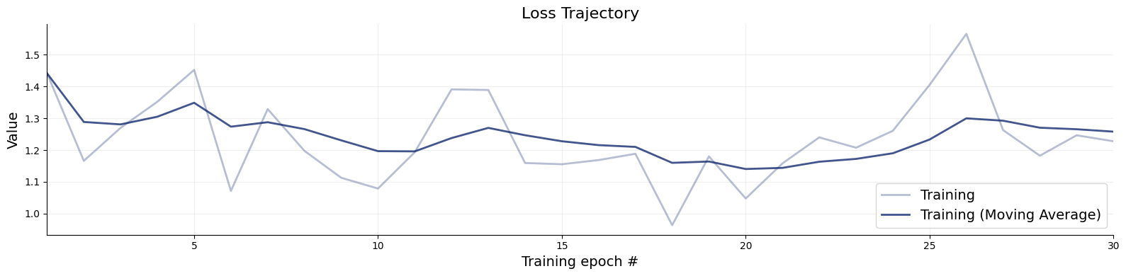
Once we defined our approximator, we can train it using simulated data.
Code
history = worfklow.fit_online(epochs=30)
Validation
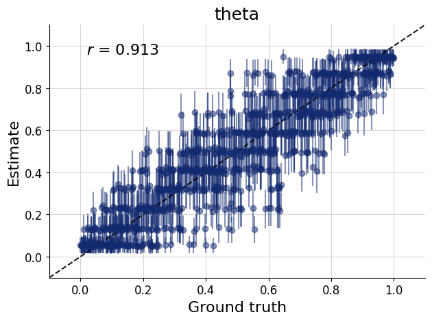
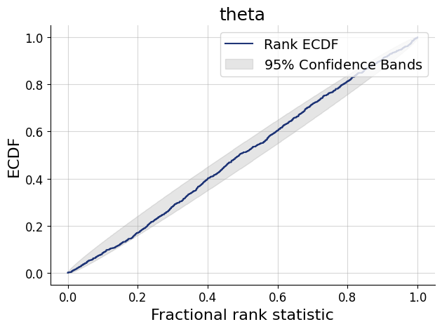
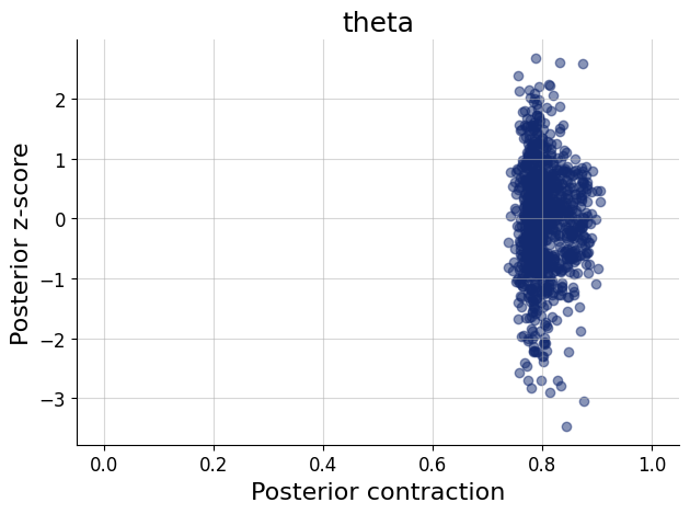
After training, we can validate our networks. The BasicWorkflow object we defined provides some basic diagnostics, which often comes in handy to conduct quick, boilerplate validation.
The basic idea of diagnostics are as follows: We first generate a batch of fresh test data from the simulator. Then, we apply our networks on these simulations, obtaining a posterior approximation for each simulated data set.
Then, we can use the simulations and predicted posteriors for model checks, such as parameter recovery, simulation-based calibration, model sensitivity, and so on. To read about these diagnostics in more depth, please refer to Schad et al. (2021) and Talts et al. (2018). Most of these diagnostics are possible to obtain with traditional (MCMC) methods as well (e.g. Kucharský et al., 2021), though it is typically very laborious to run them. ABI makes these checks very easy because inference at this stage is cheap.
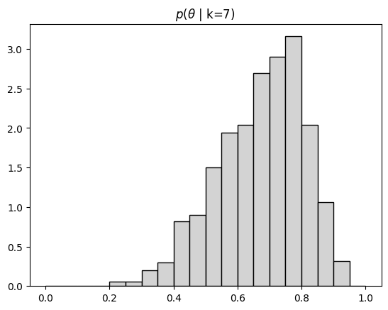
After training and validation, we use our approximator to infer the posterior distribution of \(\theta\) given observed data. Here we compute the posterior if observed 7 successes.
The data needs to be specified in the same format as produced by the simulator (except that now we will be missing the keys of the variables we are inferring, i.e., "theta").
If you managed to go through the steps above, congratulations! You have created and ran a Bayesian model using BayesFlow.
The example presented in this document is rather simple and would not be that useful in analysis of real data, as we trained a very specific model (a binomial model with fixed number of trials \(n=10\) and fixed hyperparameters of the prior distribution \(\theta \sim \text{Beta}(1, 1)\)). Since the model is so simple, we also did not use any summary network.
However, successuly running this example should give you confidence that at least BayesFlowworks on your computer. You are ready to go to the next examples.
References
Kucharský, Š., Tran, N.-H., Veldkamp, K., Raijmakers, M., & Visser, I. (2021). Hidden markov models of evidence accumulation in speeded decision tasks. Computational Brain & Behavior, 4, 416–441.
Lee, M. D., & Wagenmakers, E.-J. (2013). Bayesian CognitiveModeling: APracticalCourse. Cambridge University Press.
Schad, D. J., Betancourt, M., & Vasishth, S. (2021). Toward a principled Bayesian workflow in cognitive science. Psychological Methods, 26(1), 103.
Talts, S., Betancourt, M., Simpson, D., Vehtari, A., & Gelman, A. (2018). Validating bayesian inference algorithms with simulation-based calibration. arXiv Preprint arXiv:1804.06788.