Pearson correlation with uncertainty

Author

Šimon Kucharský

Published

May 6, 2025

Code
import os
if "KERAS_BACKEND" not in os.environ:
    # set this to "torch", "tensorflow", or "jax"
    os.environ["KERAS_BACKEND"] = "jax"

import numpy as np
import bayesflow as bf
import matplotlib.pyplot as plt
INFO:bayesflow:Using backend 'jax'

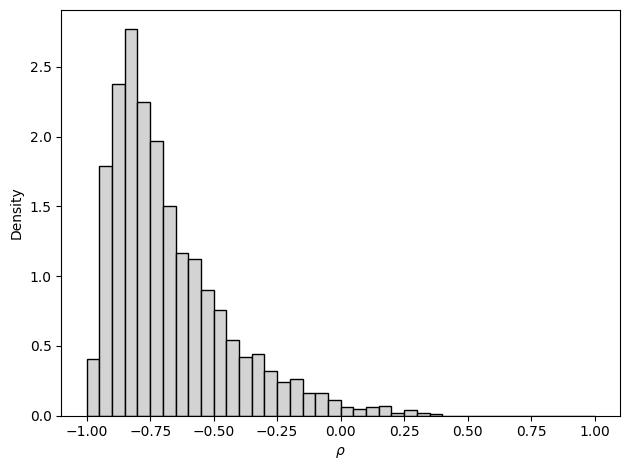
In this example we will estimate a Pearson’s correlation coefficient, assuming known reliability of measurement of the two variables. We will assume that the true variable \(y\) and measurement error \(\epsilon\) are independent and so the measurement variance is simply a sum of the true and error variances, \(\sigma_x^2 = \sigma^2 + \sigma_\epsilon^2\), and reliability is then \(a=\frac{\sigma^2}{\sigma_x^2}\).

\[\begin{equation} \begin{aligned} \rho & \sim \text{Uniform}(-1, 1) \\ \mathbb{y} & \sim \text{MvGaussian}\left((0, 0), \begin{bmatrix} \sigma_{1}^2 & \rho\sigma_{1}\sigma_{2} \\ \rho\sigma_{1}\sigma_{2} & \sigma_{2}^2\end{bmatrix} \right) \\ \mathbb{\epsilon} & \sim \text{MvGaussian}\left((0, 0), \begin{bmatrix} \sigma_{\epsilon1}^2 & \rho\sigma_{\epsilon1}\sigma_{\epsilon2} \\ \rho\sigma_{\epsilon1}\sigma_{\epsilon2} & \sigma_{\epsilon2}^2\end{bmatrix} \right) \\ x & \leftarrow y + \epsilon \\ r & \leftarrow \text{cor}(\mathbb{x}). \end{aligned} \end{equation}\]

Simulator

We will amortize over a range of sample sizes and reliabilities.

Code
def context():
    return dict(
        n = np.random.randint(5, 20),
        reliability = np.random.beta(a=5, b=2, size=2)
    )

def prior():
    return dict(rho = np.random.uniform(low=-1, high=1))

def likelihood(n, reliability, rho):
    sd_true = np.sqrt(reliability)
    sd_err = 1 - np.sqrt(reliability)

    y = np.random.multivariate_normal(
        mean=[0, 0], 
        cov=[
            [np.square(sd_true[0]), rho * np.prod(sd_true)], 
            [rho * np.prod(sd_true), np.square(sd_true[1])]], 
        size = n)
    e = np.random.normal(loc=0, scale=sd_err, size=(n, 2))
    x = y+e
    r = np.corrcoef(x[:,0], x[:,1])[0,1]

    return dict(r=r)

simulator = bf.make_simulator([context, prior, likelihood])

Approximator

We will approximate the posterior of \(\rho\) given sample size \(n\), mearuement reliabilities, and sample correlation coefficients.

Code
adapter=(
    bf.Adapter()
    .constrain("rho", lower=-1, upper=1)
    .rename("rho", "inference_variables")
    .concatenate(["n", "reliability", "r"], into="inference_conditions")
)
Code
workflow=bf.BasicWorkflow(
    simulator=simulator,
    adapter=adapter,
    inference_network=bf.networks.CouplingFlow()
)

Training

Code
history=workflow.fit_online(epochs=20, batch_size=256)

Validation

Code
test_data=simulator.sample(1000)
figs=workflow.plot_default_diagnostics(test_data=test_data, num_samples=500)

Inference

We will conduct an inference for the correlation coefficient for the data reported in Lee & Wagenmakers (2013, p. 64) of response times and IQ scores of 11 participants.

Code
rt = [0.8, 1.0, 0.5, 0.9, 0.7, 0.4, 1.2, 1.4, 0.6, 1.1, 1.3]
iq = [102, 98, 100, 105, 103, 110, 99, 87, 113, 89, 93]

r=np.corrcoef(rt, iq)[1,0]

The original example by Lee & Wagenmakers sets the measurement error to 0.03 and 1 for RTs and IQ, respectivelly. Our model is parametrized in terms of measurement reliability instead. We approximate the reliabilities using the formula \(1 - \sigma_\epsilon^2 / \sigma_x^2\). Here, \(\sigma_\epsilon\) are the values \(0.03\) and \(1\) set by Lee & Wagenmakers (2013). In the case of RTs, we approximate \(\sigma_x\) by its sample counterpart. In the case of IQ, we set it’s \(\sigma_x=15\) (since that’s how IQ tests are standardized).

Code
error_rt = 0.03
error_iq = 1
reliability = [
    1 - np.square(error_rt) / np.var(rt),
    1 - np.square(error_iq) / np.square(15)
]
reliability
[0.991, 0.9955555555555555]
Code
inference_data = dict(
    r = np.array([[r]]),
    n = np.array([[len(rt)]]),
    reliability = np.array(reliability)[np.newaxis]
)
Code
samples = workflow.sample(num_samples=2000, conditions=inference_data)
Code
plt.hist(samples["rho"].flatten(), density=True, color="lightgray", edgecolor="black", bins=np.arange(-1, 1.05, 0.05))
plt.xlabel(r"$\rho$")
plt.ylabel("Density")
plt.tight_layout()

References

Lee, M. D., & Wagenmakers, E.-J. (2013). Bayesian Cognitive Modeling: A Practical Course. Cambridge University Press.

Reuse