Inferring a rate

Author

Šimon Kucharský

Published

May 6, 2025

Code

import os

if "KERAS_BACKEND" not in os.environ:
    # set this to "torch", "tensorflow", or "jax"
    os.environ["KERAS_BACKEND"] = "jax"

import matplotlib.pyplot as plt
import numpy as np
import bayesflow as bf

INFO:bayesflow:Using backend 'jax'

The first problem in this chapter involves inferring a binomial rate:

\[\begin{equation} \begin{aligned} \theta & \sim \text{Beta}(1, 1) \\ k & \sim \text{Binomial}(\theta, n). \end{aligned} \end{equation}\]

Simulator

We will amortize over different sample sizes, so we will also draw randonly \(n\) during simulations.

Code

def context():
    return dict(n=np.random.randint(1, 101))

def prior():
    return dict(theta=np.random.beta(a=1, b=1))

def likelihood(n, theta):
    return dict(k=np.random.binomial(n=n, p=theta))

simulator=bf.make_simulator([context, prior, likelihood])

Approximator

Code

adapter = (
    bf.Adapter()
    .constrain("theta", lower=0, upper=1)
    .rename("theta", "inference_variables")
    .concatenate(["k", "n"], into="inference_conditions")
)

Code

workflow=bf.BasicWorkflow(
    simulator=simulator,
    adapter=adapter,
    inference_network=bf.networks.CouplingFlow()
)

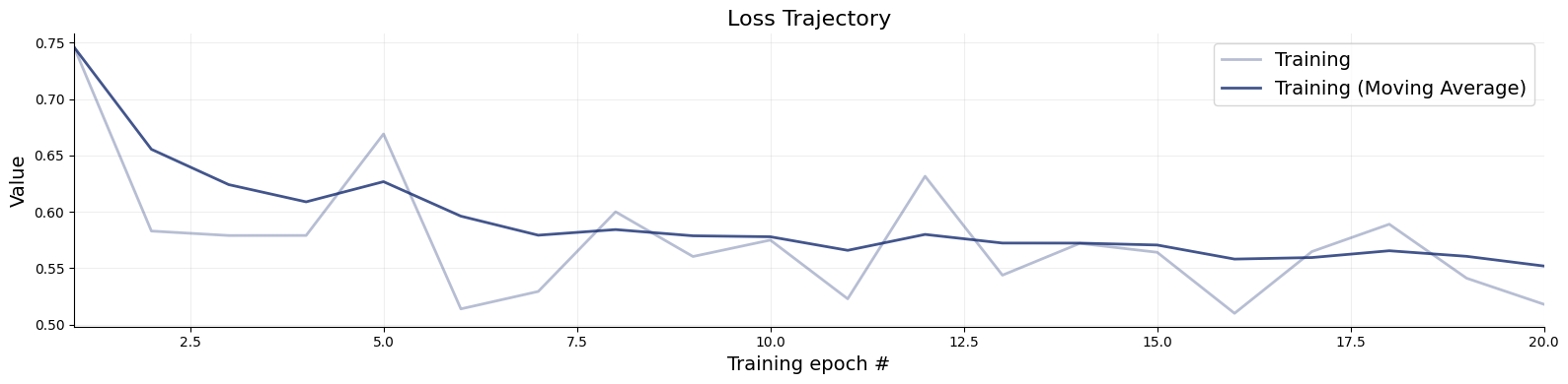
Training

Code

history=workflow.fit_online(epochs=20, batch_size=512)

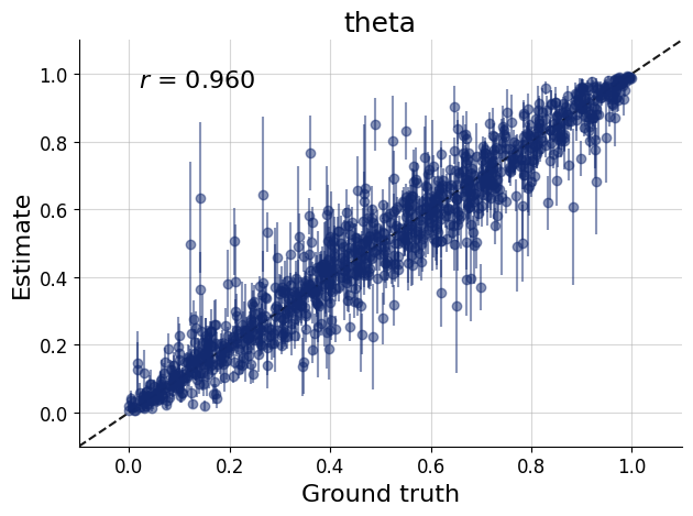
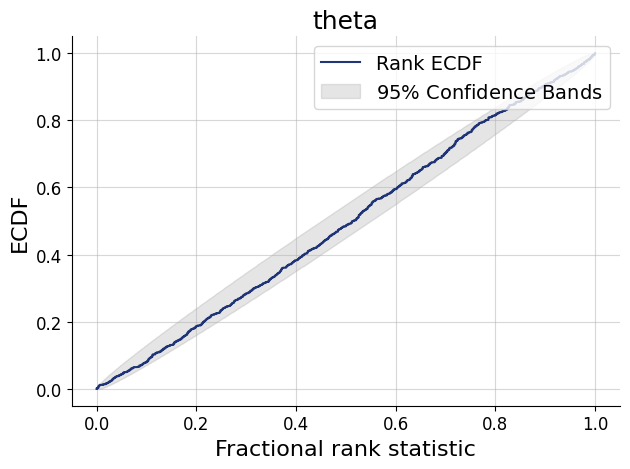
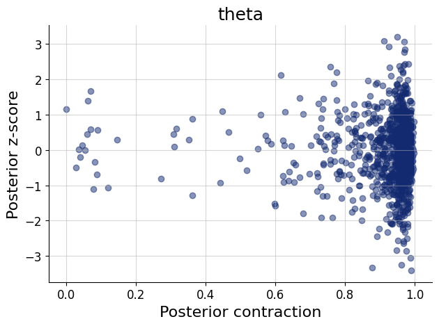
Validation

Code

test_data=simulator.sample(1000)
figs=workflow.plot_default_diagnostics(test_data=test_data, num_samples=500)

Inference

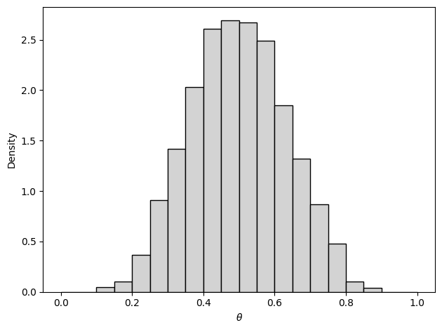
Now we obtain the approximation of the posterior distribution of \(\theta\) given \(k=5\) and \(n=10\)

Code

inference_data = dict(
    k = np.array([[5]]),
    n = np.array([[10]])
)

Code

samples = workflow.sample(num_samples=2000, conditions=inference_data)

Code

workflow.samples_to_data_frame(samples).describe()

	theta
count	2000.000000
mean	0.498038
std	0.134124
min	0.125993
25%	0.401482
50%	0.496852
75%	0.591911
max	0.870781

Code

plt.hist(samples["theta"].flatten(), density=True, color="lightgray", edgecolor="black", bins=np.arange(0, 1.05, 0.05))
plt.xlabel(r"$\theta$")
plt.ylabel("Density")
plt.tight_layout()

References

Lee, M. D., & Wagenmakers, E.-J. (2013). Bayesian Cognitive Modeling: A Practical Course. Cambridge University Press.

Reuse

CC BY NC