Difference between two rates

Author

Šimon Kucharský

Published

May 6, 2025

Code

import os

if "KERAS_BACKEND" not in os.environ:
    # set this to "torch", "tensorflow", or "jax"
    os.environ["KERAS_BACKEND"] = "jax"

import matplotlib.pyplot as plt
import numpy as np
import bayesflow as bf

INFO:bayesflow:Using backend 'jax'

In this section we will estimate the difference between two binomial rates according to the following model:

\[\begin{equation} \begin{aligned} k_1 & \sim \text{Binomial}(\theta_1, n_1) \\ k_2 & \sim \text{Binomial}(\theta_2, n_2) \\ \theta_1 & \sim \text{Beta}(1, 1) \\ \theta_2 & \sim \text{Beta}(1, 1) \\ \delta & \leftarrow \theta_1 - \theta_2 \\ \end{aligned} \end{equation}\]

Simulator

Code

def context():
    return dict(
        n=np.random.randint(1, 101, size=2)
    )

def prior():
    theta=np.random.beta(a=1, b=1, size=2)

    return dict(theta=theta, delta=theta[0]-theta[1])

def likelihood(n, theta):
    k=np.random.binomial(n=n, p=theta)

    return dict(k=k)

simulator = bf.make_simulator([context, prior, likelihood])

Approximator

Code

adapter=(
    bf.Adapter()
    .constrain("delta", lower=-1, upper=1)
    .rename("delta", "inference_variables")
    .concatenate(["k", "n"], into="inference_conditions")
)

Code

workflow=bf.BasicWorkflow(
    simulator=simulator,
    adapter=adapter,
    inference_network=bf.networks.CouplingFlow()
)

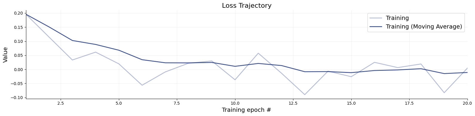
Training

Code

history=workflow.fit_online(epochs=20, batch_size=512)

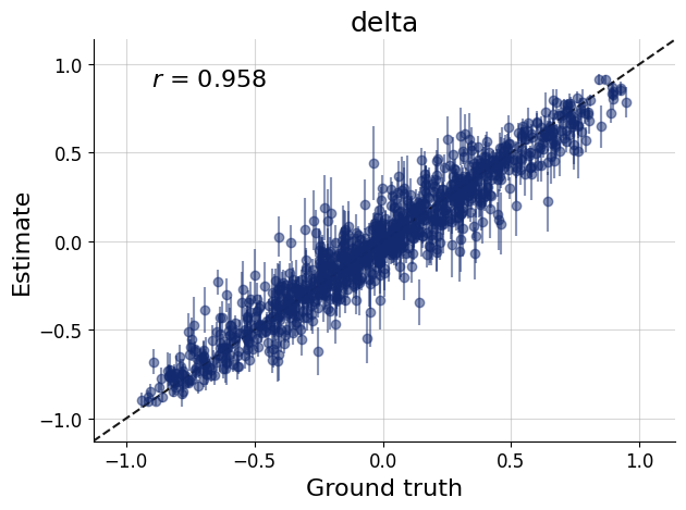
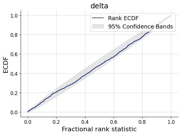
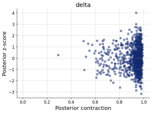
Validation

Code

test_data=simulator.sample(1000)
figs=workflow.plot_default_diagnostics(test_data=test_data, num_samples=500)

Inference

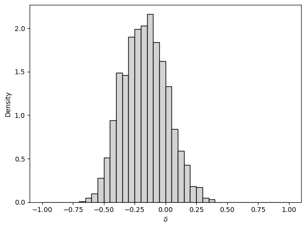
Here we estimate the parameters with \(k_1 = 5\), \(k_2 = 7\), \(n_1 = n_2 = 10\).

Code

inference_data=dict(
    k = np.array([[5, 7]]),
    n = np.array([[10, 10]])
)

Code

samples=workflow.sample(num_samples=2000, conditions=inference_data)

Code

workflow.samples_to_data_frame(samples).describe()

	delta
count	2000.000000
mean	-0.166482
std	0.178362
min	-0.659297
25%	-0.296740
50%	-0.171059
75%	-0.041115
max	0.390967

Code

plt.hist(samples["delta"].flatten(), density=True, color="lightgray", edgecolor="black", bins=np.arange(-1, 1.05, 0.05))
plt.xlabel(r"$\delta$")
plt.ylabel("Density")
plt.tight_layout()

References

Lee, M. D., & Wagenmakers, E.-J. (2013). Bayesian Cognitive Modeling: A Practical Course. Cambridge University Press.

Reuse

CC BY NC